This vignette show the comparison for a one state Categorical Functional Data (CFD) between the naive PLS, Functional PLS and Smooth PLS.
Parameters
nind = 100 # number of individuals (train set)
start = 0 # First time
end = 100 # end time

lambda_0 = 0.2 # Exponential law parameter for state 0
lambda_1 = 0.1 # Exponential law parameter for state 1
prob_start = 0.5 # Probability of starting with state 1

curve_type = 'cat'

TTRatio = 0.2 # Train Test Ratio means we have floor(nind*TTRatio/(1-TTRatio))
# individuals in the test set
NotS_ratio = 0.2 # noise variance over total variance for Y
beta_0_real=5.4321 # Intercept value for the link between X(t) and Y

nbasis = 10 # number of basis functions
norder = 4 # 4 for cubic splines basis

beta_real_func = beta_1_real_func # link between X(t) and Y

regul_time = seq(start, end, 5) # regularisation time sequence
regul_time_0 = seq(start, end, 1)

int_mode = 1 # in case of integration errors.
Data creation
df & df_test
Here we create some data to work with :
df = generate_X_df(nind = nind, start = start, end = end, curve_type = 'cat',
                   lambda_0 = lambda_0, lambda_1 = lambda_1,
                   prob_start = prob_start)

head(df)
#>   id      time state
#> 1  1  0.000000     0
#> 2  1  2.883051     1
#> 3  1 16.173600     0
#> 4  1 16.331487     1
#> 5  1 16.893597     0
#> 6  1 18.476103     1
nind_test = number_of_test_id(TTRatio = TTRatio, nind = nind)

df_test = generate_X_df(nind = nind_test, start = start, end = end,
                        curve_type = 'cat', lambda_0 = lambda_0, lambda_1 = lambda_1,
                        prob_start = prob_start)
names(df)
#> [1] "id"    "time"  "state"
print(paste0("We have ", length(unique(df_test$id)), " id on test set."))
#> [1] "We have 25 id on test set."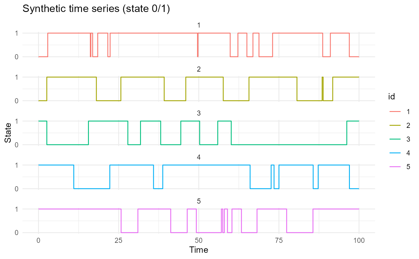
plot_CFD_individuals(df,by_cfda = TRUE)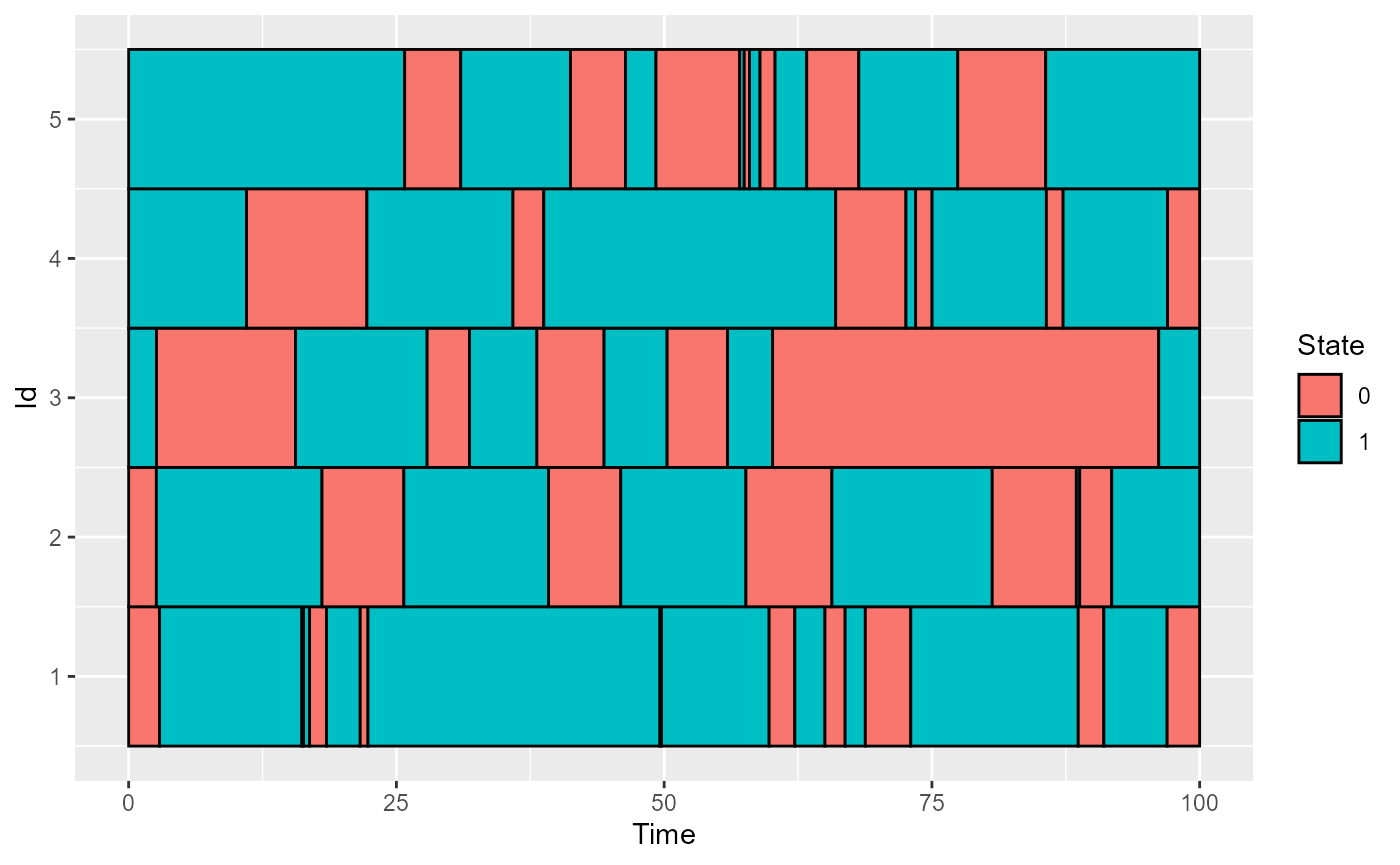
Y_df & Y_df_test
Y_df = generate_Y_df(df, curve_type = 'cat',
                     beta_real_func_or_list = beta_real_func,
                     beta_0_real, NotS_ratio, id_col = 'id', time_col = 'time')
#> Warning: package 'future' was built under R version 4.4.3

Y_df_test = generate_Y_df(df_test, curve_type = 'cat',
                          beta_real_func_or_list =  beta_real_func,
                          beta_0_real, NotS_ratio,
                          id_col = 'id', time_col = 'time')
Y = Y_df$Y_noised
names(Y_df)
#> [1] "id"       "Y_real"   "Y_noised"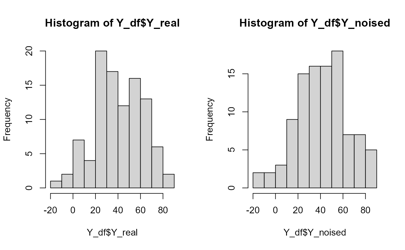
par(oldpar)Data manipulation
The following manipulation will be required form some of the following chunks.
length(regul_time)
#> [1] 21
df_regul = regularize_time_series(df, time_seq = regul_time,
                                  curve_type = curve_type)
df_wide = convert_to_wide_format(df_regul)

df_test_regul = regularize_time_series(df_test, time_seq = regul_time,
                                       curve_type = curve_type)
df_test_wide = convert_to_wide_format(df_test_regul)
Basis creation
basis = create_bspline_basis(start, end, nbasis, norder)
# ORTHOGONAL
#basis = fda::create.fourier.basis(rangeval=c(start, end), nbasis=(nbasis))
plot(basis, main=paste0(nbasis, " Function basis")) # note cubic or Fourier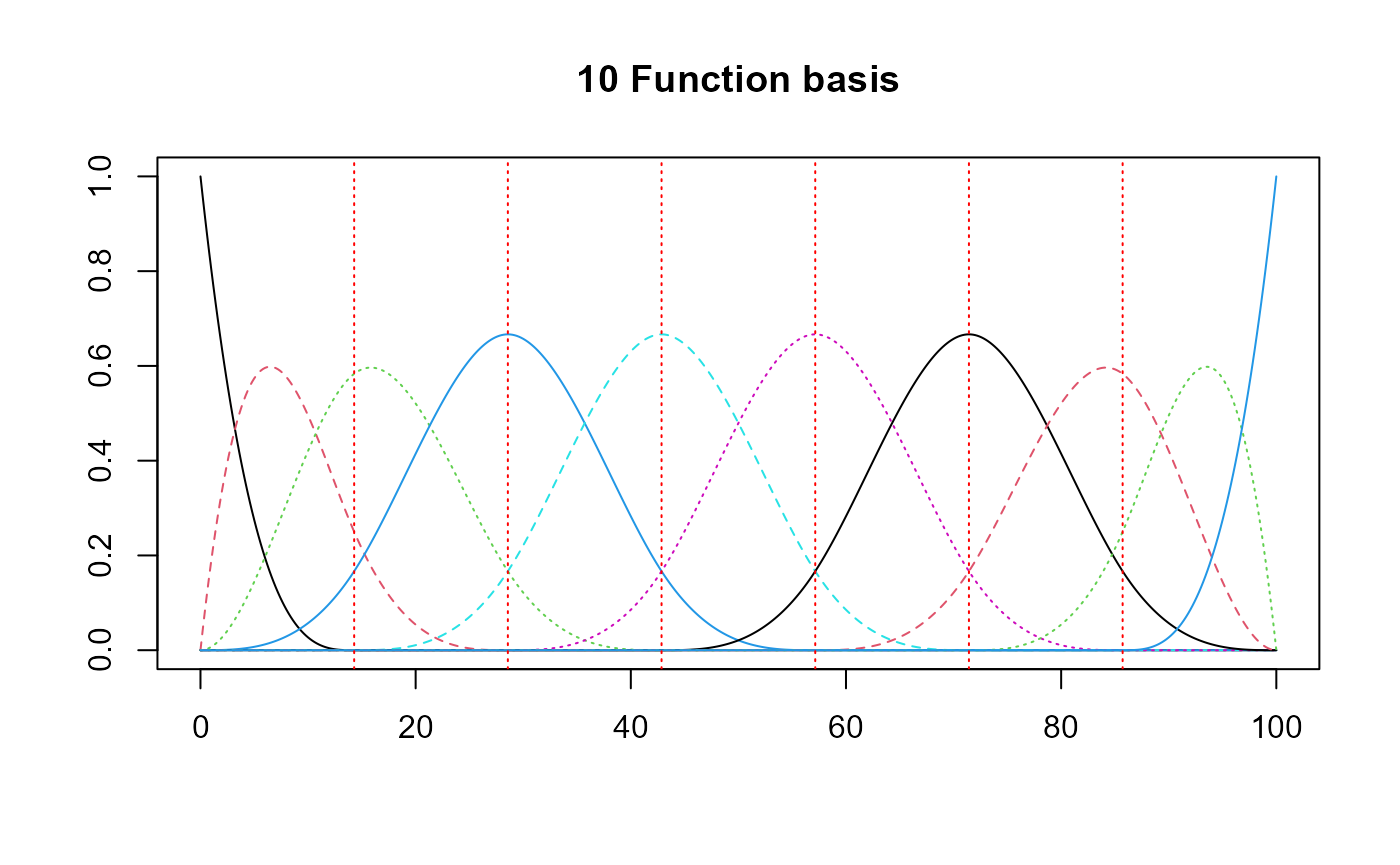
Naive PLS
Model
Here we perform the naive PLS on the data.
naive_pls_obj = naivePLS(df_list = df, Y = Y, curve_type_obj = 'cat',
                         regul_time_obj = regul_time,
                         id_col_obj = 'id', time_col_obj = 'time',
                         print_steps = TRUE, plot_rmsep = TRUE,
                         print_nbComp = TRUE, plot_reg_curves = TRUE)
#> ### Naive PLS ###
#> => Input format assertions.
#> => Input format assertions OK.
#> => Data formatting.
#> => PLS model.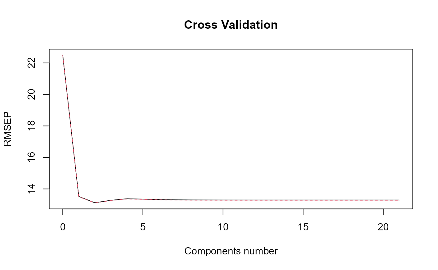
#> [1] "Optimal number of PLS components : 2"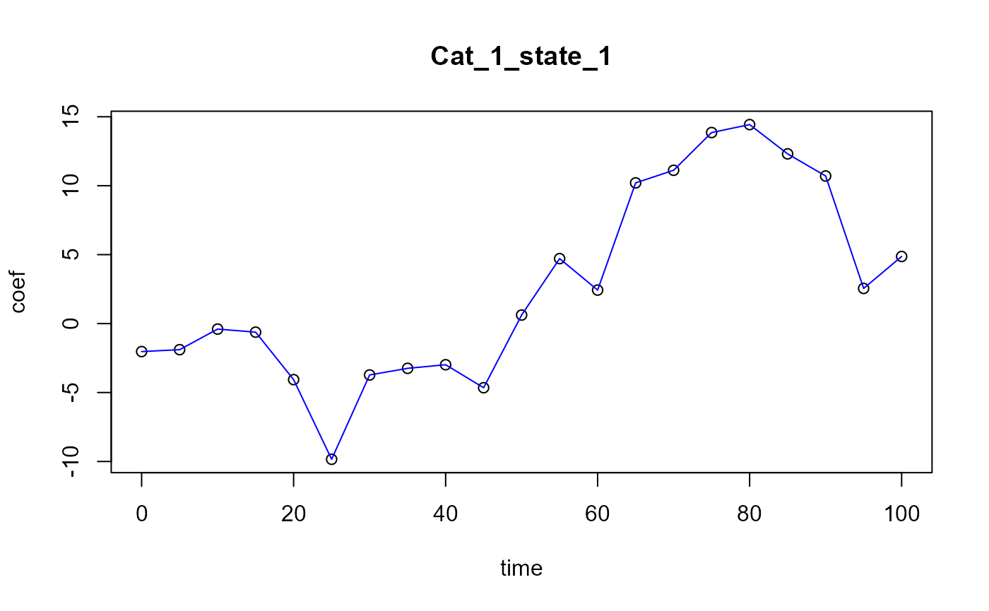
names(naive_pls_obj)
#> [1] "plsr_model"    "nbCP_opti"     "curves_names"  "opti_reg_coef"
#> [5] "reg_obj"
Regression coefficients
We can plot the coefficients :
plot(x = regul_time, y = naive_pls_obj$opti_reg_coef,
xlab='regul_time', ylab='beta coefficient value',
main="naive pls regression coefficients")
lines(x = regul_time, y = naive_pls_obj$opti_reg_coef, col='blue')
lines(x=start:end, y=beta_real_func(start:end, end), col='red')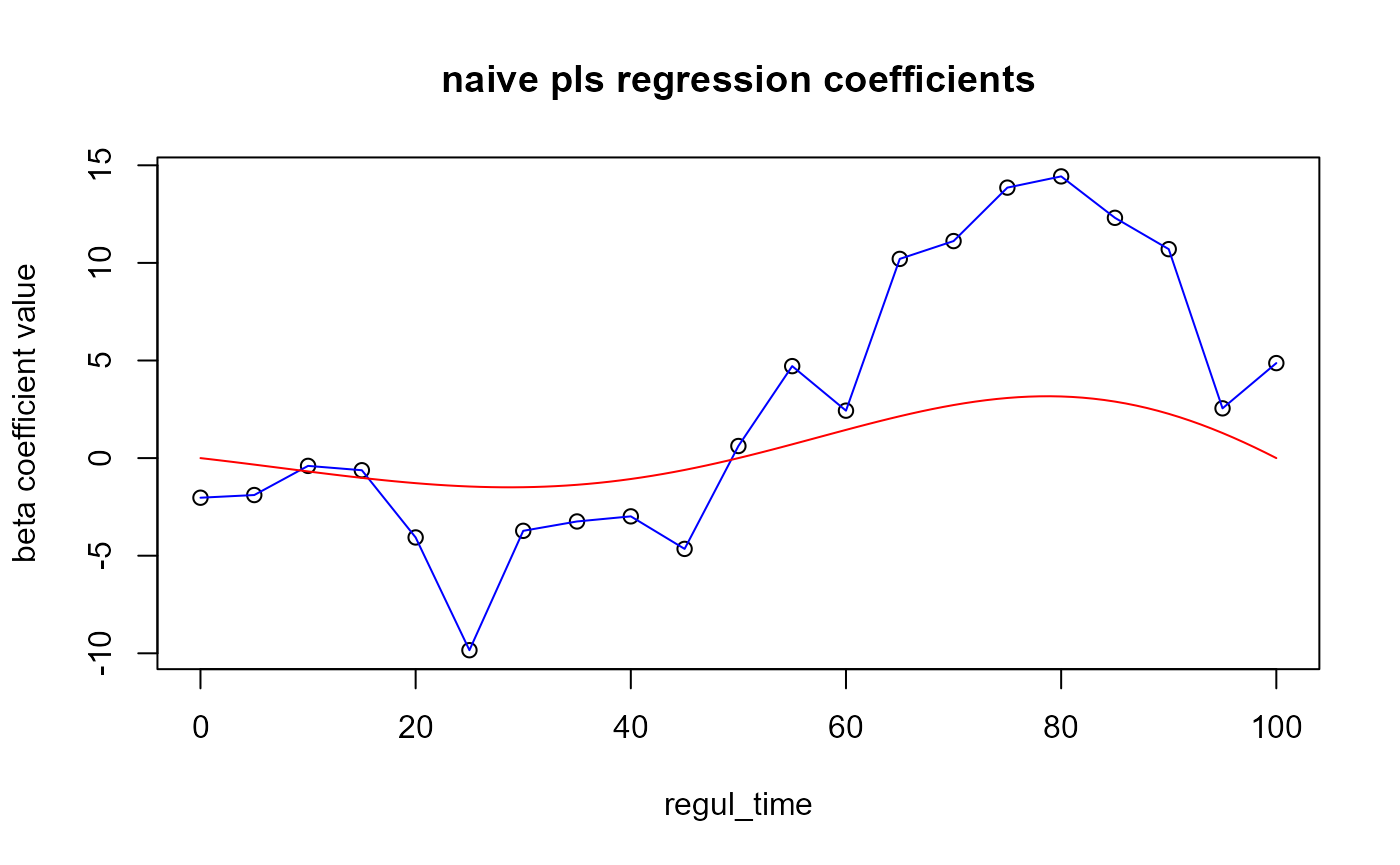 ## Results On train set :
Y_hat = predict(naive_pls_obj$plsr_model,
                ncomp = naive_pls_obj$nbCP_opti,
                newdata = as.matrix(df_wide[, -c(1)]))

cat("R^2 \n")
#> R^2
r_squared_values(Y, Y_hat)
#> [1] 0.7678782
r_squared_values(Y_df$Y_real, Y_hat)
#> [1] 0.8320421
cat("Press \n")
#> Press
press_values(Y, Y_hat)
#> [1] 11516.94
cat("RMSEP \n")
#> RMSEP
sqrt(press_values(Y, Y_hat)/nind)
#> [1] 10.7317
On test set :
Y_hat_test = predict(naive_pls_obj$plsr_model,
                     ncomp = naive_pls_obj$nbCP_opti,
                     newdata = as.matrix(df_test_wide[, -c(1)]))

cat("R^2 \n")
#> R^2
print(paste0("There is ", 100*NotS_ratio, "% of noised in Y"))
#> [1] "There is 20% of noised in Y"
cat("R^2 on Y_df_test$Y_noised \n")
#> R^2 on Y_df_test$Y_noised
r_squared_values(Y_df_test$Y_noised, Y_hat_test)
#> [1] 0.600826
cat("R^2 on Y_df_test$Y_real \n")
#> R^2 on Y_df_test$Y_real
r_squared_values(Y_df_test$Y_real, Y_hat_test)
#> [1] 0.7949041
cat("Press \n")
#> Press
press_values(Y_df_test$Y_real, Y_hat_test)
#> [1] 2230.391
cat("RMSEP \n")
#> RMSEP
sqrt(press_values(Y_df_test$Y_real, Y_hat_test)/length(Y_hat_test))
#> [1] 9.445404
FPLS
fpls_obj = funcPLS(df_list = list(df), Y = Y, basis_obj = basis,
                     regul_time_obj = regul_time, curve_type_obj = 'cat',
                     plot_rmsep = TRUE, plot_reg_curves = TRUE,
                     print_steps =TRUE)
#> ### Functional PLS ###
#> => Input format assertions.
#> => Input format assertions OK.
#> => Building alpha matrix.
#> => Building curve names.
#> ==> Evaluating alpha for : CatFD_1_state_1.
#> => Evaluate metrix and root_metric.
#> => plsr(Y ~ trans_alphas).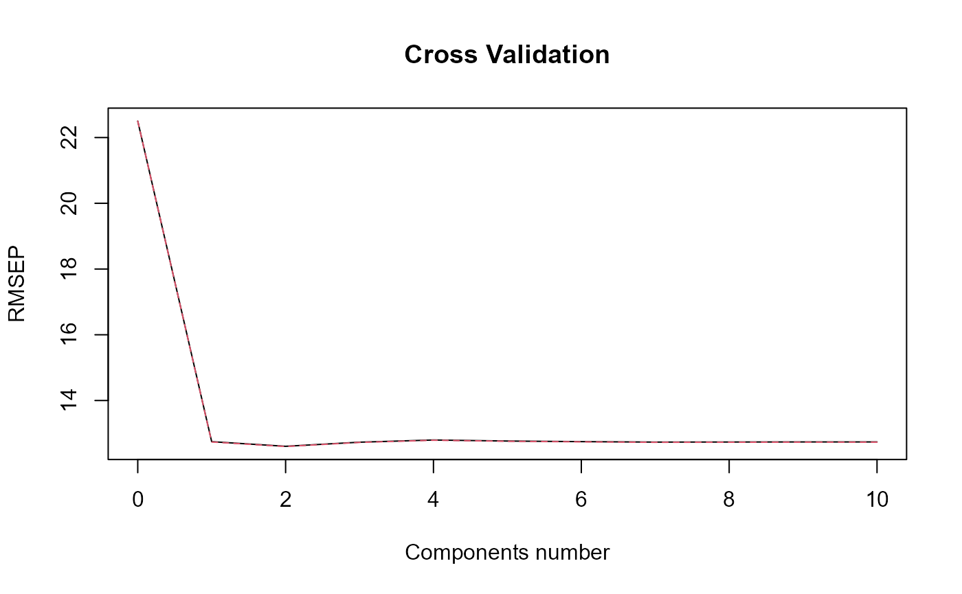
#> Optimal number of PLS components :  2 .
#> => Build Intercept and regression curves for optimal number of components.
#>  ==> Build  regression curve for : CatFD_1_state_1
y_lim = eval_max_min_y(f_list = list(beta_real_func,
                                     fpls_obj$reg_obj$CatFD),
                       regul_time = regul_time_0)

plot(regul_time_0, beta_real_func(regul_time_0), type='l', xlab="Beta_t",
     ylim = c(-2, 3.5))
plot(fpls_obj$reg_obj$CatFD, add=TRUE, col='red')
#> [1] "done"
legend("topleft",
         legend = c("delta_FPLS"),
         col = c("red"),
         lty = 1,
         lwd = 1)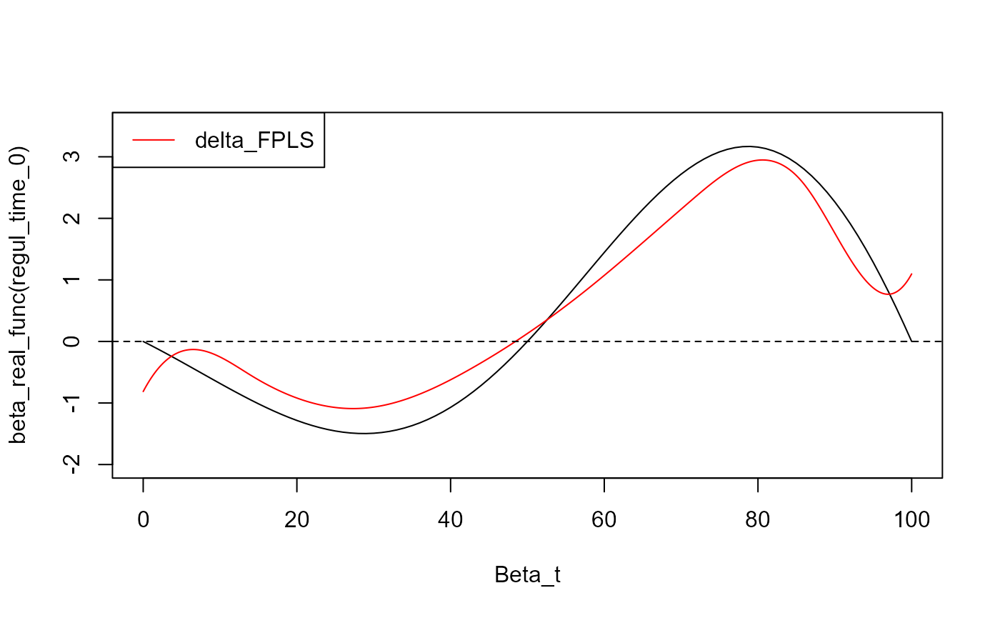
Result
Y_hat_fpls = (predict(fpls_obj$plsr_model, ncomp = fpls_obj$nbCP_opti,
                newdata = fpls_obj$trans_alphas)
              + fpls_obj$reg_obj$Intercept
              + mean(Y))

sqrt(press_values(Y_df$Y_real, Y_hat_fpls)/length(Y_hat_fpls))
#> [1] 48.49346
sqrt(press_values(Y_df$Y_noised, Y_hat_fpls)/length(Y_hat_fpls))
#> [1] 48.21771

cat("NotS_ratio \n")
#> NotS_ratio
print(paste0("There is ", 100*NotS_ratio, "% of noise in Y"))
#> [1] "There is 20% of noise in Y"
cat("R^2 on Y_df_test$Y_noised \n")
#> R^2 on Y_df_test$Y_noised
r_squared_values(Y_df$Y_noised, Y_hat_fpls)
#> [1] -3.685889
cat("R^2 on Y_df_test$Y_real \n")
#> R^2 on Y_df_test$Y_real
r_squared_values(Y_df$Y_real, Y_hat_fpls)
#> [1] -4.428922
Y_hat_fpls_test = smoothPLS_predict(df_predict = df_test,
                                    delta_list = fpls_obj$reg_obj,
                                    curve_type = curve_type,
                                    regul_time_obj = regul_time)

sqrt(press_values(Y_df_test$Y_real, Y_hat_fpls_test)/length(Y_hat_fpls_test))
#> [1] 3.945121
sqrt(press_values(Y_df_test$Y_noised, Y_hat_fpls_test)/length(Y_hat_fpls_test))
#> [1] 10.27909

cat("R^2 \n")
#> R^2
print(paste0("There is ", 100*NotS_ratio, "% of noise in Y"))
#> [1] "There is 20% of noise in Y"
cat("R^2 on Y_df_test$Y_noised \n")
#> R^2 on Y_df_test$Y_noised
r_squared_values(Y_df_test$Y_noised, Y_hat_fpls_test)
#> [1] 0.730098
cat("R^2 on Y_df_test$Y_real \n")
#> R^2 on Y_df_test$Y_real
r_squared_values(Y_df_test$Y_real, Y_hat_fpls_test)
#> [1] 0.9642203
Smooth PLS
spls_obj = smoothPLS(df_list = df, Y = Y, basis_obj = basis,
                     curve_type_obj = 'cat', orth_obj = TRUE, int_mode = 1,
                     print_steps = TRUE, print_nbComp = TRUE,
                     plot_rmsep = TRUE, plot_reg_curves = TRUE,
                     id_col_obj = 'id',time_col_obj = 'time',
                     jackknife = TRUE, validation = 'LOO',
                     parallel=FALSE)
#> ### Smooth PLS ###
#> => Input format assertions.
#> => Input format assertions OK.
#> => Orthonormalize basis.
#> => Data objects formatting.
#> => Evaluate Lambda matrix.
#> ==> Lambda for : CatFD_1_state_1.
#> => PLSR model.
#> => Optimal number of PLS components : 2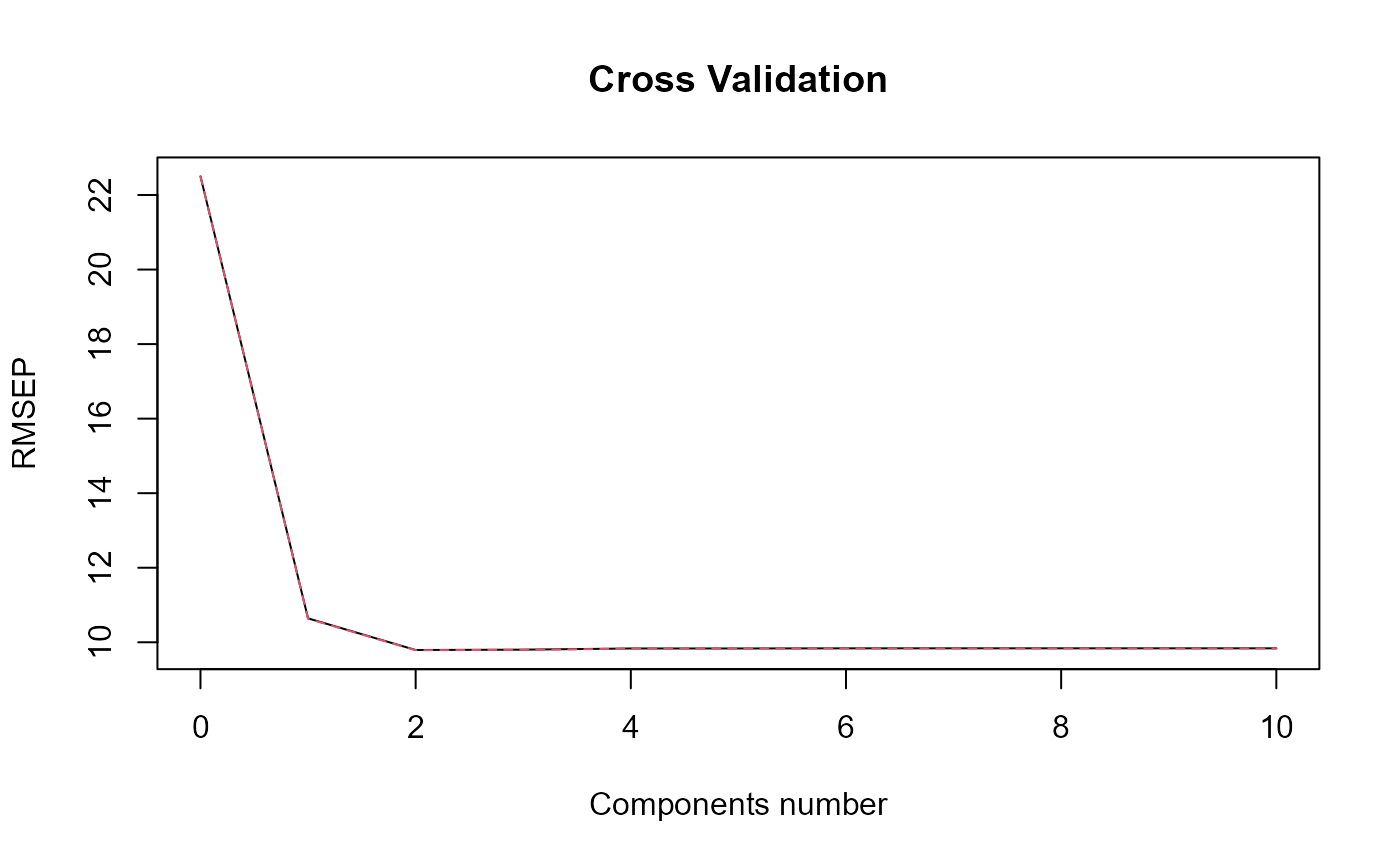
#> => Evaluate SmoothPLS functions and <w_i, p_j> coef.
#> => Build regression functions and intercept.
#> ==> Build regression curve for : CatFD_1_state_1
## delta Delta Smooth_PLS
delta_0 = spls_obj$reg_obj$Intercept
delta_0
#> [1] -0.2851742

delta = spls_obj$reg_obj$CatFD_1_state_1
plot(delta)
#> [1] "done"
y_lim = eval_max_min_y(f_list = list(beta_real_func,
                                     delta),
                       regul_time = regul_time_0)

plot(regul_time_0, beta_real_func(regul_time_0), type='l', xlab="Beta_t",
     ylim = c(-2, 3.5))
plot(delta, add=TRUE, col='blue')
#> [1] "done"
legend("topleft",
         legend = c("delta_SmoothPLS"),
         col = c("blue"),
         lty = 1,
         lwd = 1)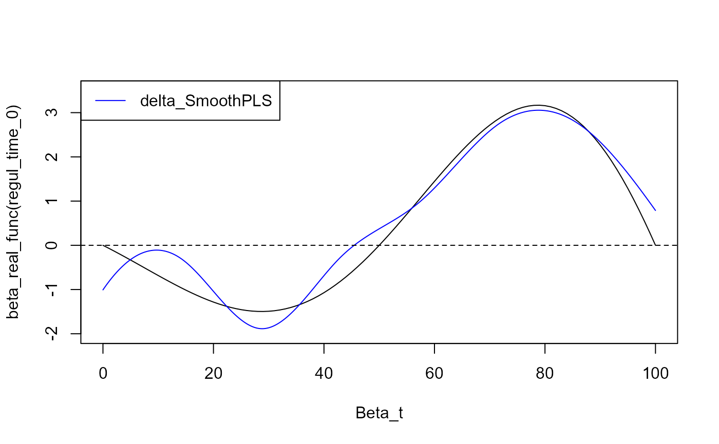
Results
#delta_0_spls
Y_hat_spls = smoothPLS_predict(df_predict = df,
                               delta_list = list(delta_0, delta),
                               curve_type = 'cat', regul_time_obj = regul_time,
                               int_mode = int_mode)


sqrt(press_values(Y_df$Y_real, Y_hat_spls)/length(Y_hat_spls))
#> [1] 3.127829
sqrt(press_values(Y_df$Y_noised, Y_hat_spls)/length(Y_hat_spls))
#> [1] 8.926796

cat("R^2 \n")
#> R^2
print(paste0("There is ", 100*NotS_ratio, "% of noise in Y"))
#> [1] "There is 20% of noise in Y"
cat("R^2 on Y_df_test$Y_noised \n")
#> R^2 on Y_df_test$Y_noised
r_squared_values(Y_df$Y_noised, Y_hat_spls)
#> [1] 0.8393909
cat("R^2 on Y_df_test$Y_real \n")
#> R^2 on Y_df_test$Y_real
r_squared_values(Y_df$Y_real, Y_hat_spls)
#> [1] 0.9774143
Y_hat_spls_test = smoothPLS_predict(df_predict = df_test,
                                    delta_list = list(delta_0, delta),
                                    curve_type = curve_type,
                                    regul_time_obj = regul_time,
                                    int_mode = int_mode)


sqrt(press_values(Y_df_test$Y_real, Y_hat_spls)/length(Y_hat_spls_test))
#> [1] 47.52298
sqrt(press_values(Y_df_test$Y_noised, Y_hat_spls)/length(Y_hat_spls_test))
#> [1] 46.99441

cat("R^2 \n")
#> R^2
print(paste0("There is ", 100*NotS_ratio, "% of noise in Y"))
#> [1] "There is 20% of noise in Y"
cat("R^2 on Y_df_test$Y_noised \n")
#> R^2 on Y_df_test$Y_noised
r_squared_values(Y_df_test$Y_noised, Y_hat_spls_test)
#> [1] 0.7219523
cat("R^2 on Y_df_test$Y_real \n")
#> R^2 on Y_df_test$Y_real
r_squared_values(Y_df_test$Y_real, Y_hat_spls_test)
#> [1] 0.9839068
Curve comparison
cat("curve_1 : smooth PLS regression curve.\n")
#> curve_1 : smooth PLS regression curve.
cat("curve_2 : functional PLS regression curve.\n")
#> curve_2 : functional PLS regression curve.
cat("curve_3 : naive PLS regression coefficients\n")
#> curve_3 : naive PLS regression coefficients

evaluate_curves_distances(real_f = beta_real_func,
                          regul_time = regul_time,
                          fun_fd_list = list(
                            delta,
                            fpls_obj$reg_obj$CatFD,
                            approxfun(x = regul_time,
                                      y = naive_pls_obj$opti_reg_coef)
                            )
                          )
#> [1] "real_f -> curve_1 / INPROD  : -8.64690065515022 / DIST : 3.62140840065327"
#> [1] "real_f -> curve_2 / INPROD  : -1.60878829989084 / DIST : 4.33943943908411"
#> [1] "real_f -> curve_3 / INPROD  : -212.658700236693 / DIST : 58.3398953923996"
y_lim = eval_max_min_y(f_list = list(spls_obj$reg_obj$CatFD_1_state_1,
                                     fpls_obj$reg_obj$CatFD_1_state_1,
                                     approxfun(x = regul_time,
                                               y = naive_pls_obj$opti_reg_coef),
                                     beta_real_func ),
                         regul_time = regul_time_0)

plot(regul_time_0, beta_real_func(regul_time_0), col = 'black',
     ylim = y_lim, xlab = 'Time', ylab = 'Value', type = 'l')
lines(regul_time_0, approxfun(x = regul_time,
                              y = naive_pls_obj$opti_reg_coef)(regul_time_0),
      col = 'green')
title(paste0(names(spls_obj$reg_obj)[2], " regression curves"))
plot(spls_obj$reg_obj$CatFD_1_state_1, col = 'blue', add = TRUE)
#> [1] "done"
plot(fpls_obj$reg_obj$CatFD_1_state_1, col = 'red', add = TRUE)
#> [1] "done"
legend("topleft",
       legend = c("Real curve", "NaivePLS coef",
                  "SmoothPLS reg curve", "FunctionalPLS reg curve"),
       col = c("black", "green", "blue", "red"),
       lty = 1,
       lwd = 1)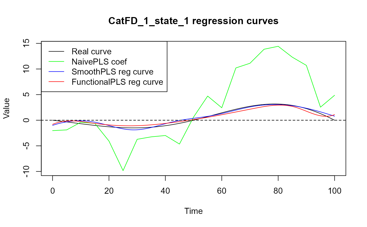
y_lim = eval_max_min_y(f_list = list(spls_obj$reg_obj$CatFD_1_state_1,
                                     fpls_obj$reg_obj$CatFD_1_state_1,
                                     beta_real_func ),
                         regul_time = regul_time_0)

plot(regul_time_0, beta_real_func(regul_time_0), type='l', ylab="Values",
     xlab = 'Time', ylim = y_lim, col = 'black')
title(paste0(names(spls_obj$reg_obj)[2], " regression curves"))
plot(spls_obj$reg_obj$CatFD_1_state_1, add=TRUE, col='blue')
#> [1] "done"
plot(fpls_obj$reg_obj$CatFD_1_state_1, add=TRUE, col='red')
#> [1] "done"
legend("topleft",
         legend = c("Real curve", "SmoothPLS", "FuncPLS"),
         col = c("black", "blue", "red"),
         lty = 1,
         lwd = 1)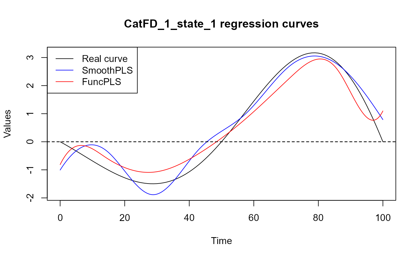
Plot the second derivatives for the smoothness :
plot(fda::deriv.fd(expr = delta, Lfdobj = 2), col='blue')
#> [1] "done"
plot(fda::deriv.fd(expr = fpls_obj$reg_obj$CatFD, Lfdobj = 2),
     add=TRUE, col='red')
#> [1] "done"
title("Second derivatives")
legend("bottomleft",
         legend = c("delta_SmoothPLS''", "delta_FPLS''"),
         col = c("blue", "red"),
         lty = 1,
         lwd = 1)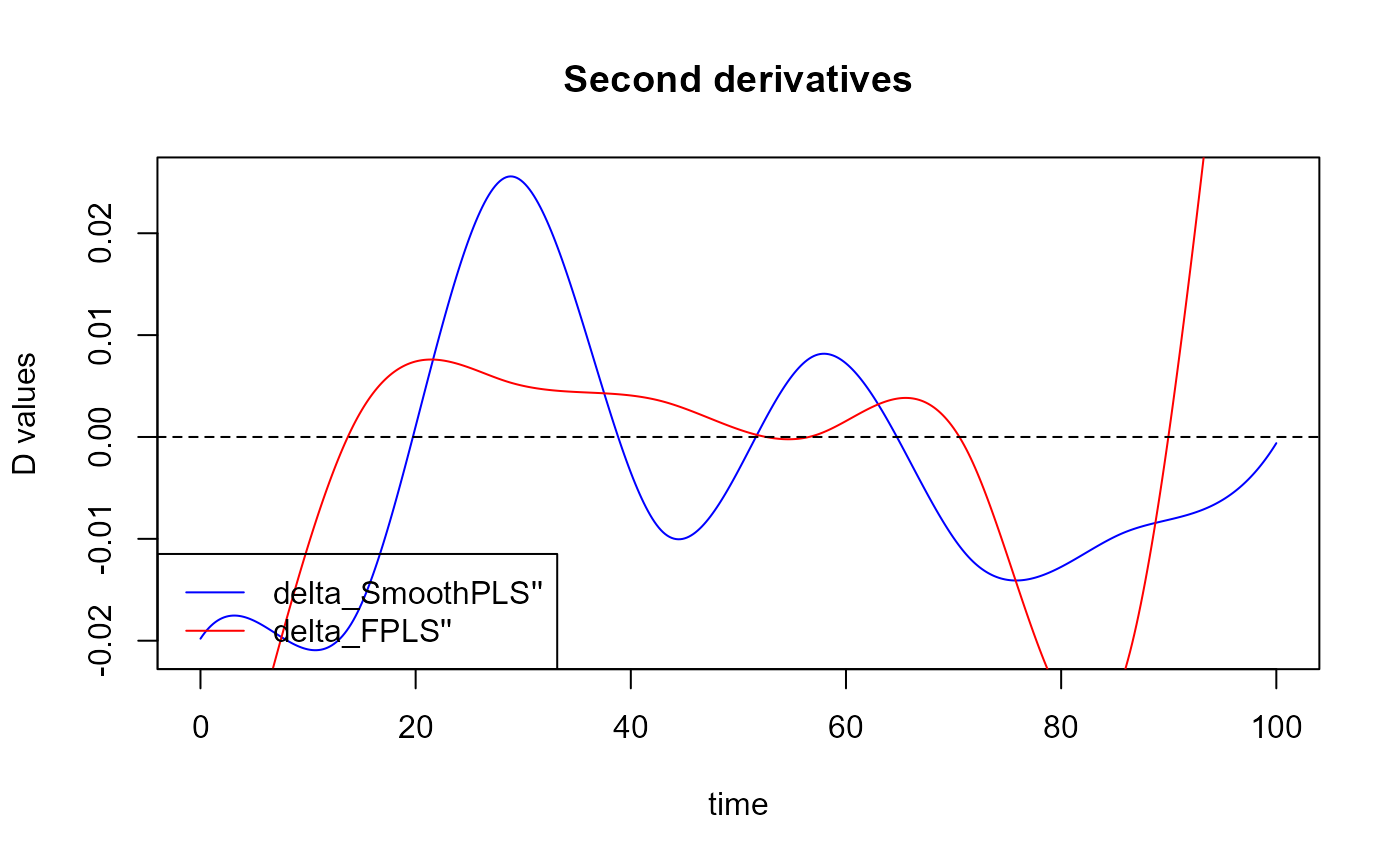
Results
train_results = data.frame(matrix(ncol = 5, nrow = 3))
colnames(train_results) = c("PRESS", "RMSE", "MAE", "R2", "var_Y")
rownames(train_results) = c("NaivePLS", "FPLS", "SmoothPLS")

test_results = train_resultsTrain set
Y_train = Y_df$Y_noised

# Naive
Y_hat = predict(naive_pls_obj$plsr_model,
                ncomp = naive_pls_obj$nbCP_opti,
                newdata = as.matrix(df_wide[, -c(1)]))
train_results["NaivePLS", ] = evaluate_results(Y_train, Y_hat)


# FPLS
Y_hat_fpls = (predict(fpls_obj$plsr_model, ncomp = fpls_obj$nbCP_opti,
                newdata = fpls_obj$trans_alphas)
              + fpls_obj$reg_obj$Intercept
              + mean(Y))

Y_hat_fpls = smoothPLS_predict(df_predict = df,
                               delta_list = fpls_obj$reg_obj,
                               curve_type = curve_type,
                               regul_time_obj = regul_time,
                               int_mode = int_mode)

train_results["FPLS", ] = evaluate_results(Y_train, Y_hat_fpls)

# Smooth PLS
Y_hat_spls = smoothPLS_predict(df_predict = df,
                               delta_list = list(delta_0, delta),
                               curve_type = 'cat',
                               regul_time_obj = regul_time,
                               int_mode = int_mode)

train_results["SmoothPLS", ] = evaluate_results(Y_train, Y_hat_spls)

train_results["NaivePLS", "nb_cp"] = naive_pls_obj$nbCP_opti
train_results["FPLS", "nb_cp"] = fpls_obj$nbCP_opti
train_results["SmoothPLS", "nb_cp"] = spls_obj$nbCP_opti
train_results
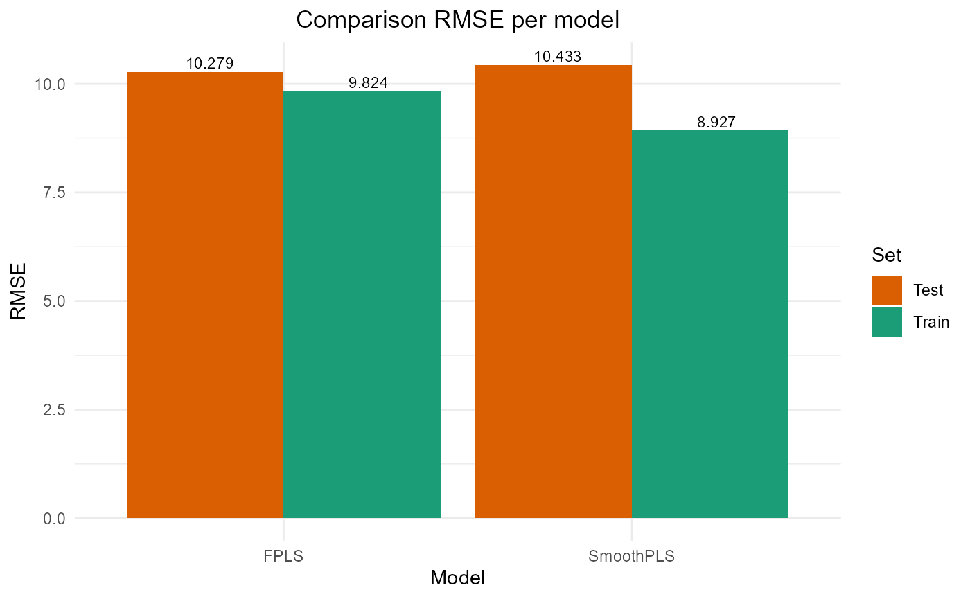
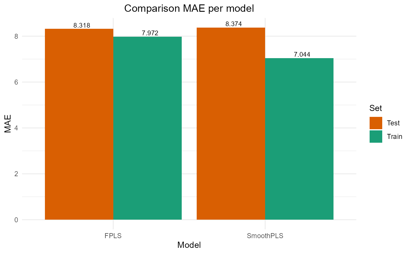
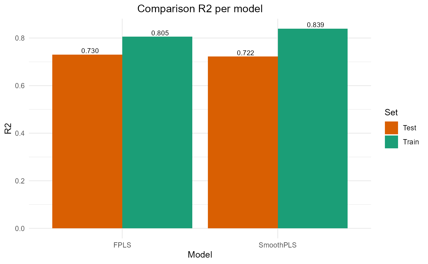
#> PRESS RMSE MAE R2 var_Y nb_cp
#> NaivePLS 11516.938 10.731700 8.899796 0.7678782 76.78782 2
#> FPLS 9650.888 9.823893 7.972429 0.8054881 61.72924 2
#> SmoothPLS 7968.769 8.926796 7.044480 0.8393909 84.17329 2
par(oldpar)Test set
Y_test = Y_df_test$Y_noised

# Naive
Y_hat = naivePLS_predict(naive_pls_obj = naive_pls_obj,
                         df_predict_list = df_test,
                         regul_time_obj = regul_time,
                         curve_type_obj = 'cat')
test_results["NaivePLS", ] = evaluate_results(Y_test, Y_hat)

# FPLS
Y_hat_fpls = smoothPLS_predict(df_predict = df_test,
                               delta_list = fpls_obj$reg_obj,
                               curve_type = curve_type,
                               regul_time_obj = regul_time,
                               int_mode = int_mode)

test_results["FPLS", ] = evaluate_results(Y_test, Y_hat_fpls)

# Smooth PLS
Y_hat_spls = smoothPLS_predict(df_predict = df_test,
                               delta_list = list(delta_0, delta),
                               curve_type = curve_type,
                               regul_time_obj = regul_time,
                               int_mode = int_mode)

test_results["SmoothPLS", ] = evaluate_results(Y_test, Y_hat_spls)

test_results["NaivePLS", "nb_cp"] = naive_pls_obj$nbCP_opti
test_results["FPLS", "nb_cp"] = fpls_obj$nbCP_opti
test_results["SmoothPLS", "nb_cp"] = spls_obj$nbCP_opti
Y_hat_naivePLS = naivePLS_predict(naive_pls_obj = naive_pls_obj,
                                  df_predict_list = df_test,
                                  regul_time_obj = regul_time,
                                  curve_type_obj = 'cat')
test_results
#>              PRESS     RMSE       MAE        R2     var_Y nb_cp
#> NaivePLS  3906.659 12.50065 10.269340 0.6008260  89.90318     2
#> FPLS      2641.492 10.27909  8.317701 0.7300980  80.29085     2
#> SmoothPLS 2721.213 10.43305  8.373668 0.7219523 109.83704     2
par(oldpar)Results plots
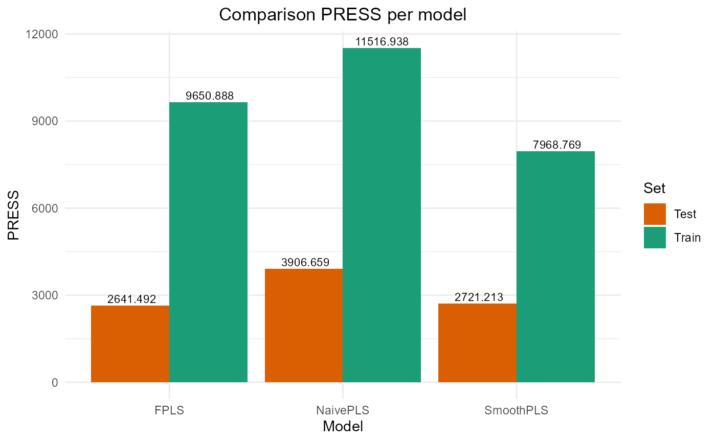
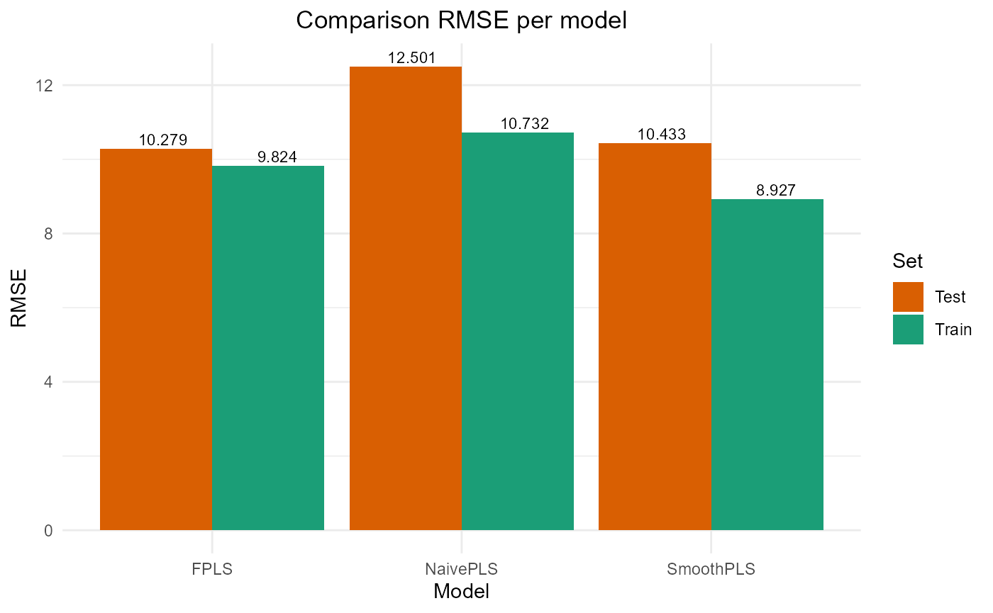
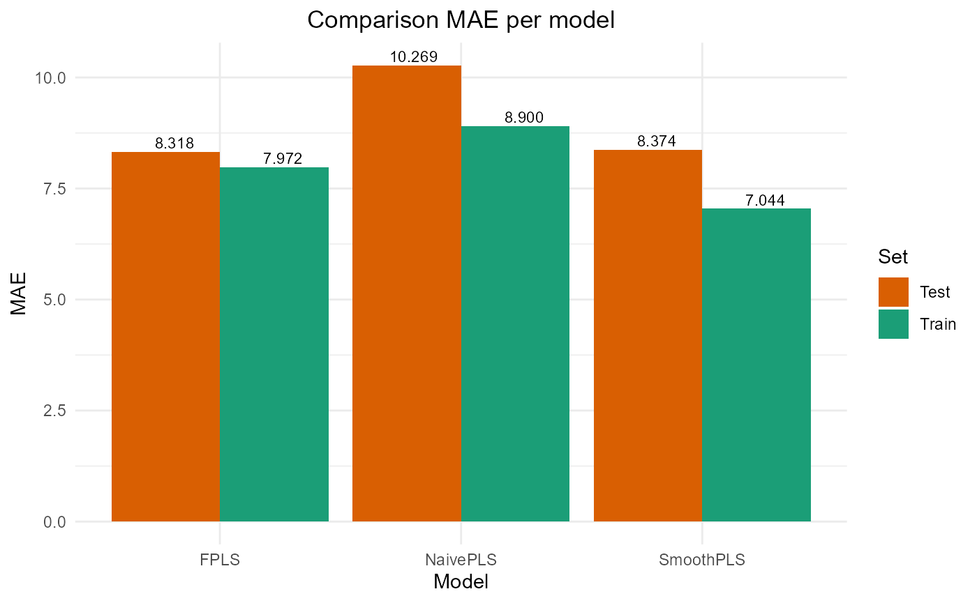
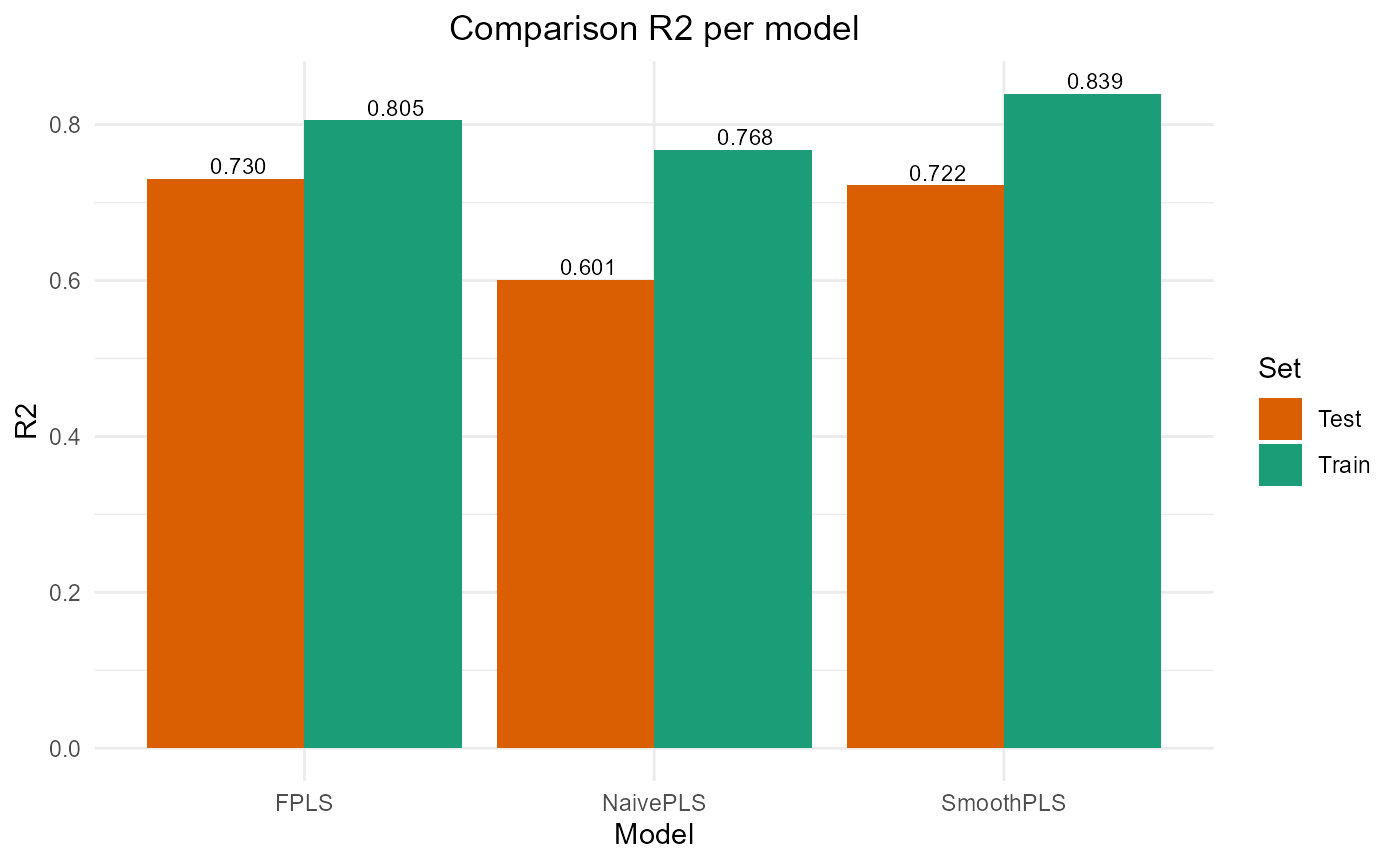
FPLS & SmoothPLS
plot_model_metrics_base(train_results, test_results,
                        models_to_plot = c('FPLS', 'SmoothPLS'))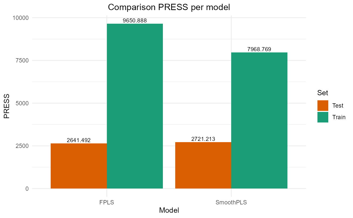
Fourier basis test
basis_f = fda::create.fourier.basis(rangeval=c(start, end), nbasis=(nbasis))
plot(basis_f, main=paste0(nbasis, " Function basis")) # note cubic or Fourier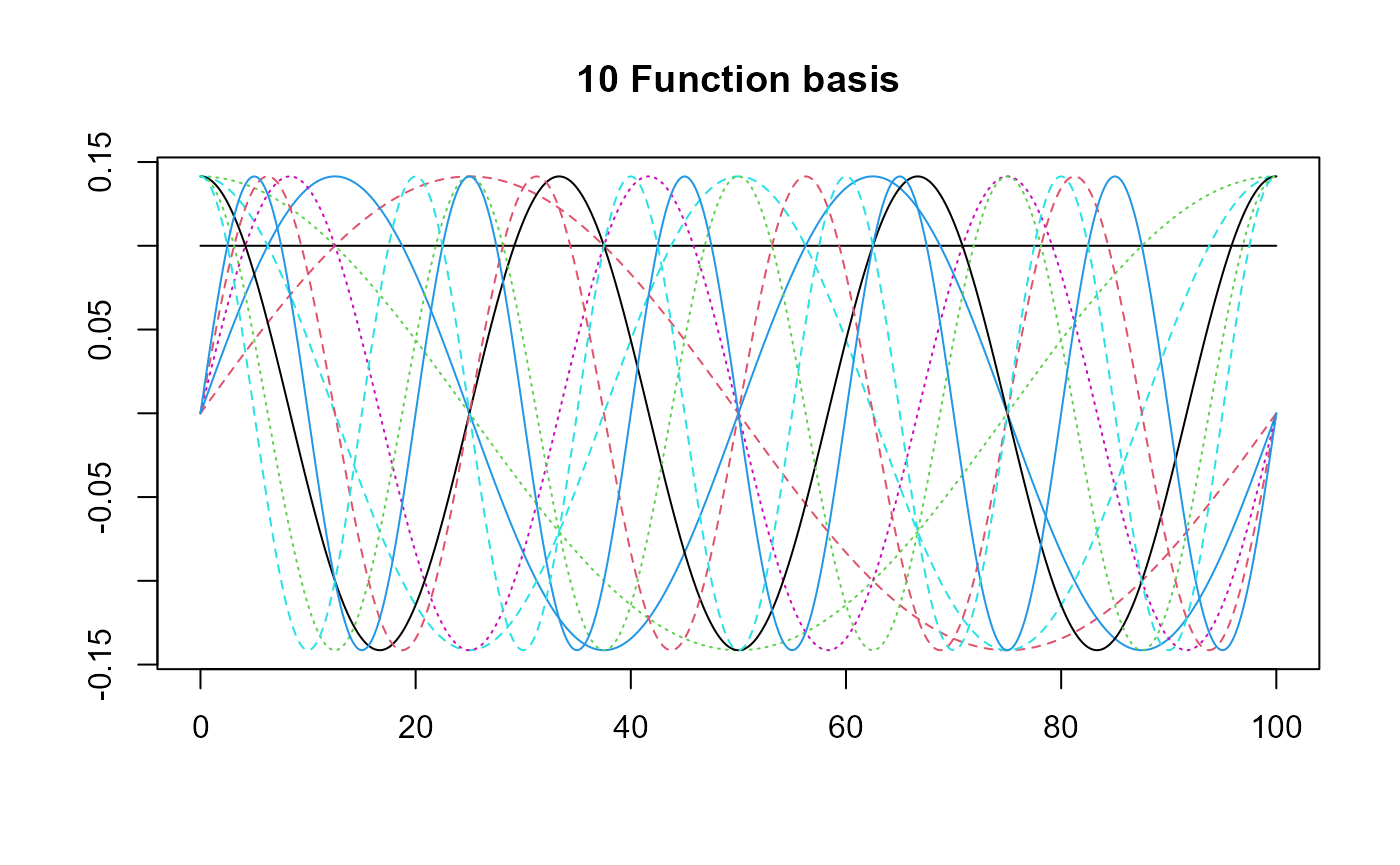
FPLS
fpls_obj_2 = funcPLS(df_list = df, Y = Y, basis_obj = basis_f,
                     regul_time_obj = regul_time, curve_type_obj = curve_type,
                     print_steps = TRUE, plot_rmsep = TRUE,
                     print_nbComp = TRUE, plot_reg_curves = TRUE)
#> ### Functional PLS ###
#> => Input format assertions.
#> => Input format assertions OK.
#> => Building alpha matrix.
#> => Building curve names.
#> ==> Evaluating alpha for : CatFD_1_state_1.
#> => Evaluate metrix and root_metric.
#> => plsr(Y ~ trans_alphas).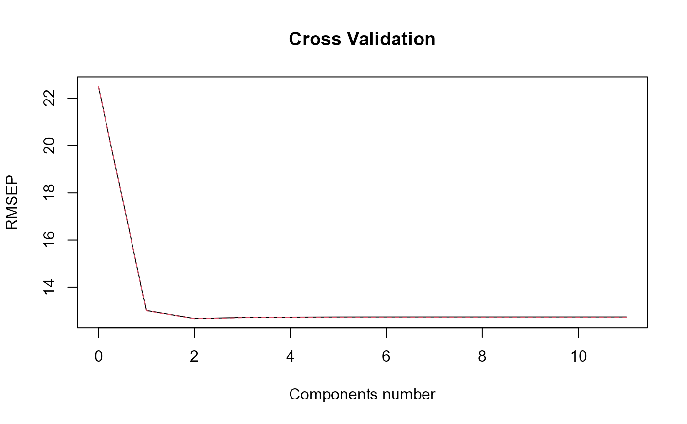
#> Optimal number of PLS components :  2 .
#> => Build Intercept and regression curves for optimal number of components.
#>  ==> Build  regression curve for : CatFD_1_state_1
Smooth PLS
spls_obj_2 = smoothPLS(df_list = df, Y = Y, basis_obj = basis_f,
                       orth_obj = FALSE, curve_type_obj = curve_type,
                       print_steps = TRUE, plot_rmsep = TRUE,
                       print_nbComp = TRUE, plot_reg_curves = TRUE)
#> ### Smooth PLS ###
#> ## Use parallelization in case of heavy computational load. ##
#> ## Threshold can be manualy adjusted : (default 2500) ##
#> ## >options(SmoothPLS.parallel_threshold = 500) ##
#> => Input format assertions.
#> => Input format assertions OK.
#> => Orthonormalize basis.
#> => Data objects formatting.
#> => Evaluate Lambda matrix.
#> ==> Lambda for : CatFD_1_state_1.
#> => PLSR model.
#> => Optimal number of PLS components : 3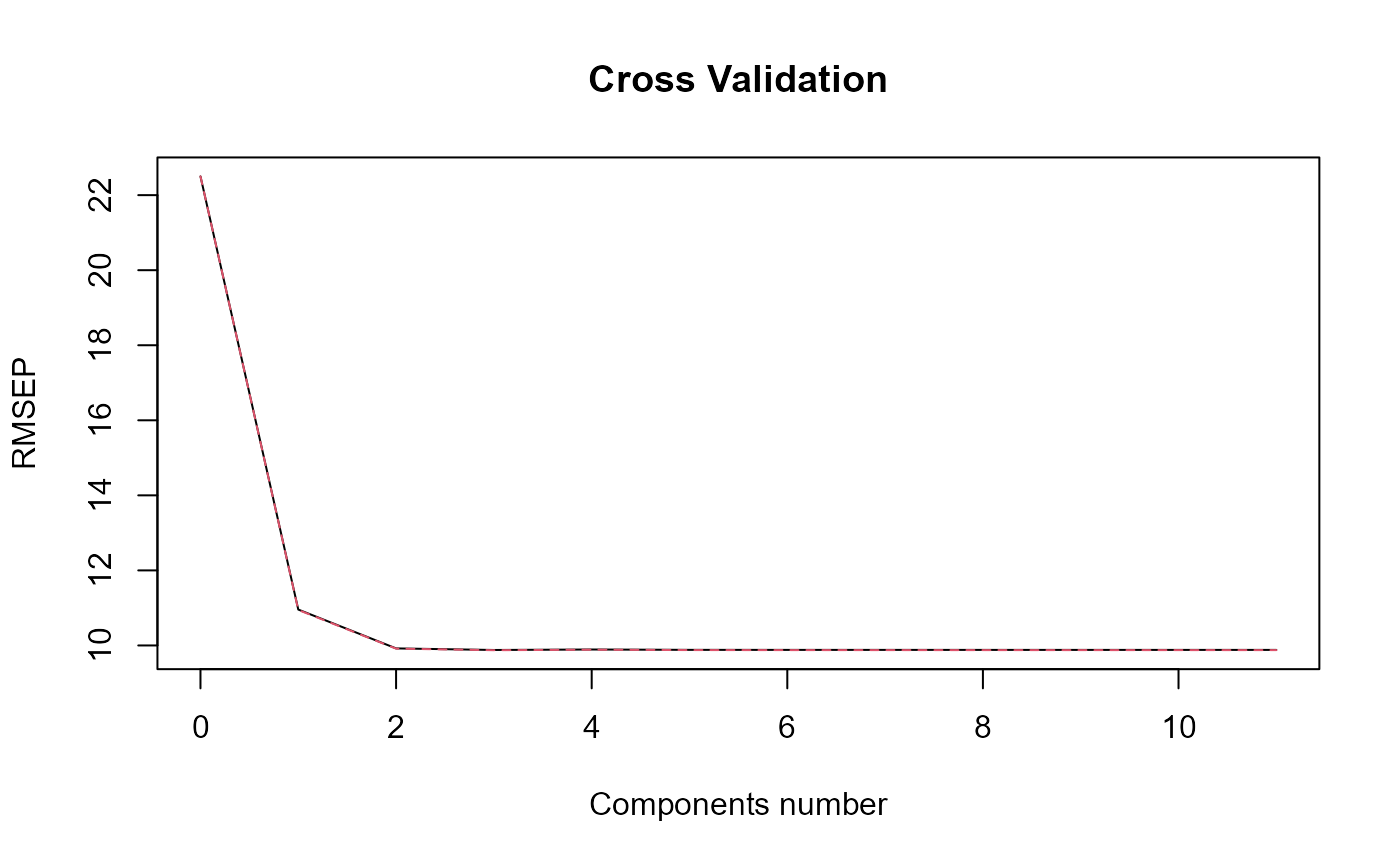
#> => Evaluate SmoothPLS functions and <w_i, p_j> coef.
#> => Build regression functions and intercept.
#> ==> Build regression curve for : CatFD_1_state_1
delta_0_2 = spls_obj_2$reg_obj$Intercept

delta_2 = spls_obj_2$reg_obj$CatFD_1_state_1
plot(delta_2)
#> [1] "done"Curve comparison
plot(regul_time_0, beta_real_func(regul_time_0), type='l', xlab="Beta_t",
     ylim = c(-2, 3.5))
plot(delta_2, add=TRUE, col='blue')
#> [1] "done"
plot(fpls_obj_2$reg_obj$CatFD, add=TRUE, col='red')
#> [1] "done"
legend("topleft",
         legend = c("delta_SmoothPLS", "delta_FPLS"),
         col = c("blue", "red"),
         lty = 1,
         lwd = 1)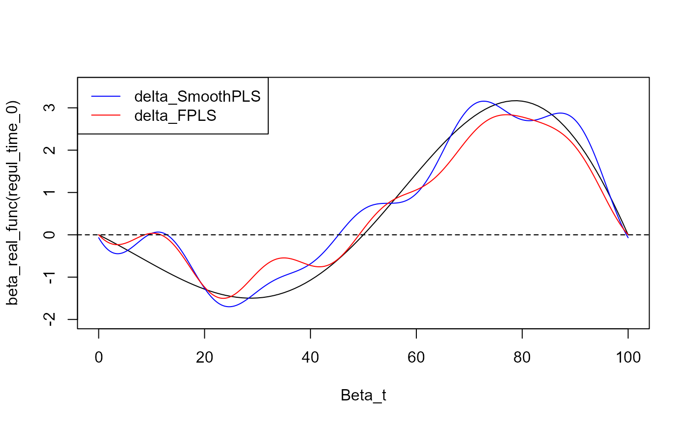
evaluate_curves_distances(real_f = beta_real_func,
                          regul_time = regul_time,
                          fun_fd_list = list(delta_2,
                                             fpls_obj_2$reg_obj$CatFD))
#> [1] "real_f -> curve_1 / INPROD  : -14.7996269337727 / DIST : 3.80924706990471"
#> [1] "real_f -> curve_2 / INPROD  : -3.71157039027193 / DIST : 4.03448526199711"
cat("curve_1 : smooth PLS regression curve.\n")
#> curve_1 : smooth PLS regression curve.
cat("curve_2 : functional PLS regression curve.\n")
#> curve_2 : functional PLS regression curve.
cat("curve_3 : naive PLS regression coefficients\n")
#> curve_3 : naive PLS regression coefficients

evaluate_curves_distances(real_f = beta_real_func,
                          regul_time = regul_time,
                          fun_fd_list = list(
                            spls_obj_2$reg_obj$CatFD_1_state_1,
                            fpls_obj_2$reg_obj$CatFD_1_state_1,
                            approxfun(x = regul_time,
                                      y = naive_pls_obj$opti_reg_coef)
                            )
                          )
#> [1] "real_f -> curve_1 / INPROD  : -14.7996269337727 / DIST : 3.80924706990471"
#> [1] "real_f -> curve_2 / INPROD  : -3.71157039027193 / DIST : 4.03448526199711"
#> [1] "real_f -> curve_3 / INPROD  : -212.658700236693 / DIST : 58.3398953923996"
y_lim = eval_max_min_y(f_list = list(spls_obj_2$reg_obj$CatFD_1_state_1,
                                     fpls_obj_2$reg_obj$CatFD_1_state_1,
                                     approxfun(x = regul_time,
                                               y = naive_pls_obj$opti_reg_coef),
                                     beta_real_func ),
                         regul_time = regul_time_0)

plot(regul_time_0, beta_real_func(regul_time_0), col = 'black',
     ylim = y_lim, xlab = 'Time', ylab = 'Value', type = 'l')
lines(regul_time_0, approxfun(x = regul_time,
                              y = naive_pls_obj$opti_reg_coef)(regul_time_0),
      col = 'green')
title(paste0(names(spls_obj_2$reg_obj)[2], " regression curves"))
plot(spls_obj_2$reg_obj$CatFD_1_state_1, col = 'blue', add = TRUE)
#> [1] "done"
plot(fpls_obj_2$reg_obj$CatFD_1_state_1, col = 'red', add = TRUE)
#> [1] "done"
legend("topleft",
       legend = c("Real curve", "NaivePLS coef",
                  "SmoothPLS reg curve", "FunctionalPLS reg curve"),
       col = c("black", "green", "blue", "red"),
       lty = 1,
       lwd = 1)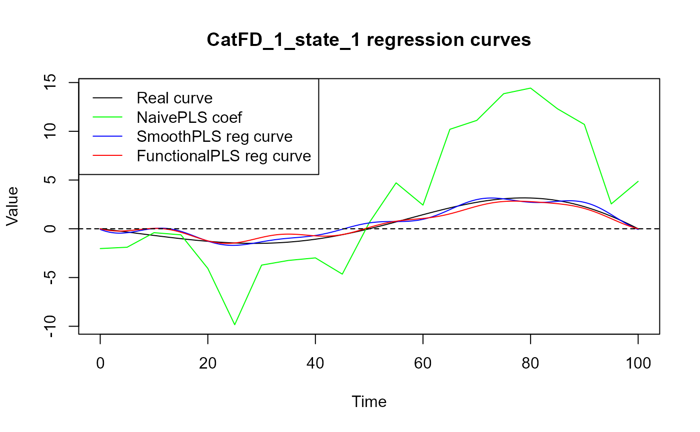
y_lim = eval_max_min_y(f_list = list(spls_obj_2$reg_obj$CatFD_1_state_1,
                                     fpls_obj_2$reg_obj$CatFD_1_state_1,
                                     beta_real_func),
                         regul_time = regul_time_0)

plot(regul_time_0, beta_real_func(regul_time_0), type='l', ylab="Values",
     xlab = 'Time', ylim = y_lim, col = 'black')
title(paste0(names(spls_obj_2$reg_obj)[2], " regression curves"))
plot(spls_obj_2$reg_obj$CatFD_1_state_1, add=TRUE, col='blue')
#> [1] "done"
plot(fpls_obj_2$reg_obj$CatFD_1_state_1, add=TRUE, col='red')
#> [1] "done"
legend("topleft",
         legend = c("Real curve", "SmoothPLS", "FuncPLS"),
         col = c("black", "blue", "red"),
         lty = 1,
         lwd = 1)
Results
train_results_f = data.frame(matrix(ncol = 5, nrow = 3))
colnames(train_results_f) = c("PRESS", "RMSE", "MAE", "R2", "var_Y")
rownames(train_results_f) = c("NaivePLS", "FPLS", "SmoothPLS")

test_results_f = train_results_fTrain set
Y_train = Y_df$Y_noised

# Naive
Y_hat = predict(naive_pls_obj$plsr_model,
                ncomp = naive_pls_obj$nbCP_opti,
                newdata = as.matrix(df_wide[, -c(1)]))
train_results_f["NaivePLS", ] = evaluate_results(Y_train, Y_hat)


# FPLS
Y_hat_fpls = (predict(fpls_obj_2$plsr_model, ncomp = fpls_obj_2$nbCP_opti,
                newdata = fpls_obj_2$trans_alphas)
              + fpls_obj_2$reg_obj$Intercept
              + mean(Y))

train_results_f["FPLS", ] = evaluate_results(Y_train, Y_hat_fpls)

# Smooth PLS
Y_hat_spls = smoothPLS_predict(df_predict_list = df,
                               delta_list = list(delta_0_2, delta_2),
                               curve_type = 'cat',
                               int_mode = int_mode)

train_results_f["SmoothPLS", ] = evaluate_results(Y_train, Y_hat_spls)

train_results_f["NaivePLS", "nb_cp"] = naive_pls_obj$nbCP_opti
train_results_f["FPLS", "nb_cp"] = fpls_obj$nbCP_opti
train_results_f["SmoothPLS", "nb_cp"] = spls_obj$nbCP_opti
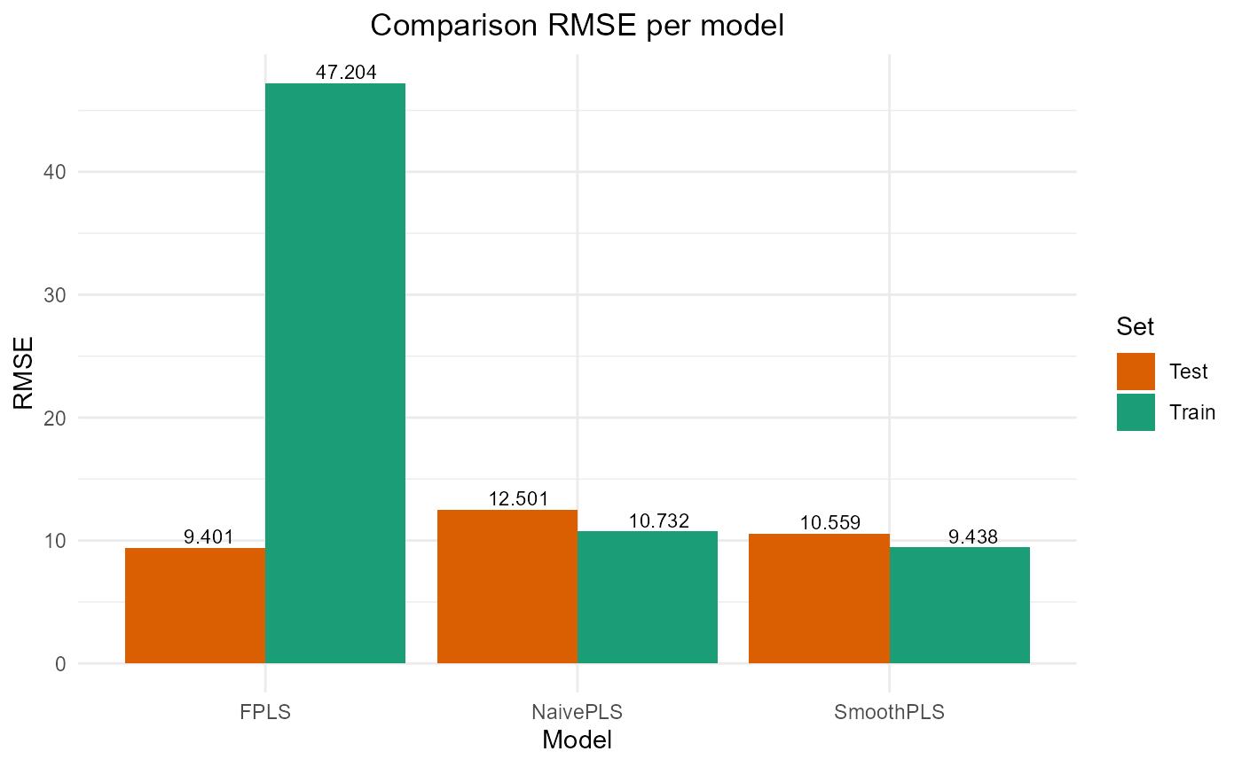
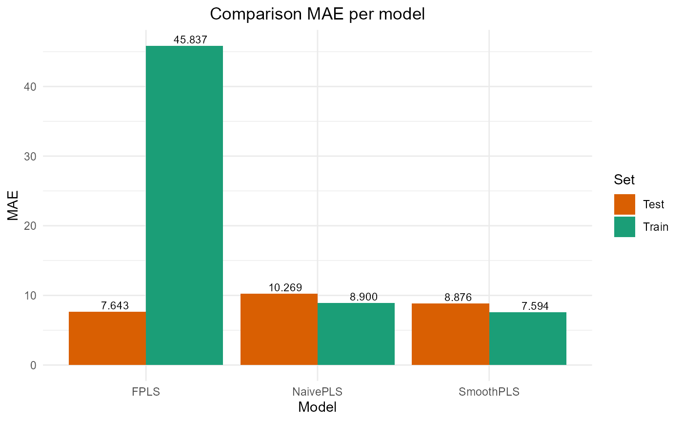
train_results_f
#> PRESS RMSE MAE R2 var_Y nb_cp
#> NaivePLS 11516.938 10.73170 8.899796 0.7678782 76.78782 2
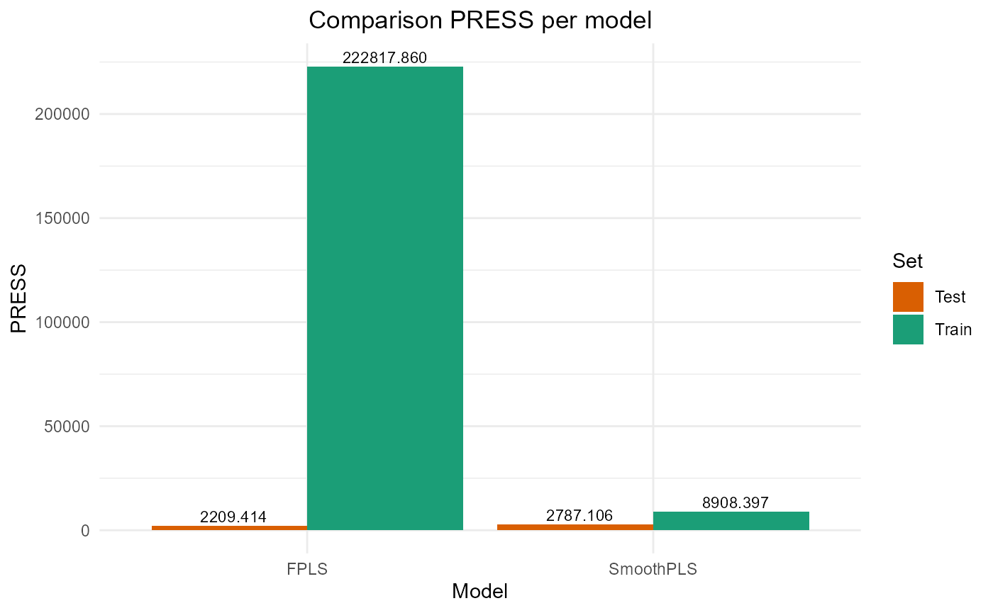
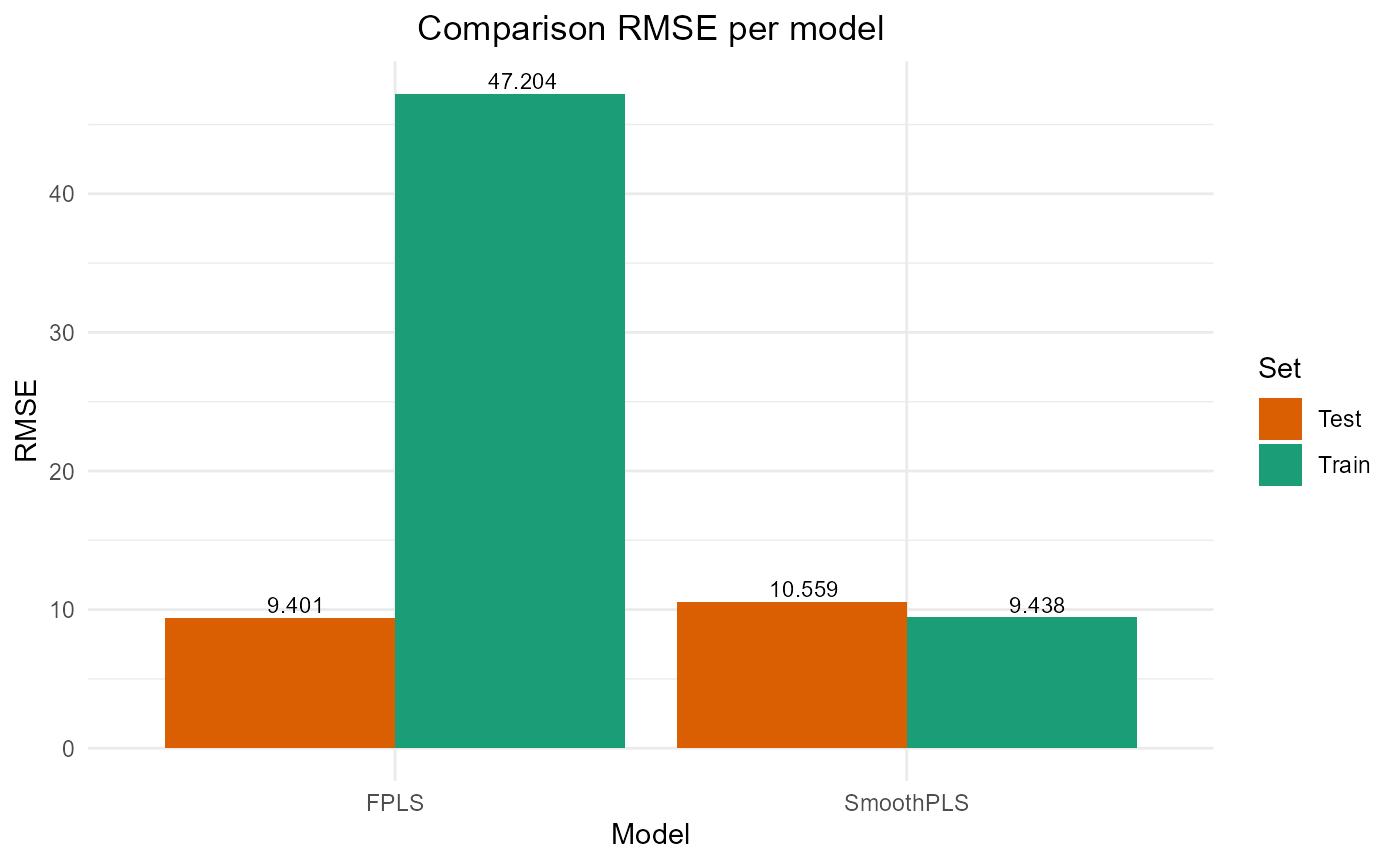
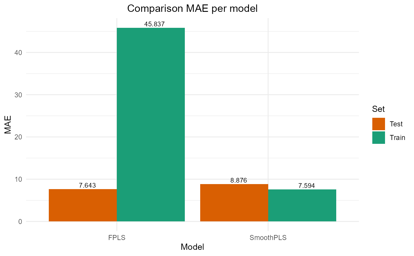
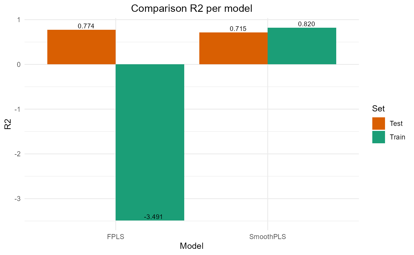
#> FPLS 222817.860 47.20359 45.837142 -3.4908532 74.37618 2
#> SmoothPLS 8908.397 9.43843 7.593621 0.8204529 82.27065 2Test set
Y_test = Y_df_test$Y_noised

# Naive
Y_hat = predict(naive_pls_obj$plsr_model,
                ncomp = naive_pls_obj$nbCP_opti,
                newdata = as.matrix(df_test_wide[, -c(1)]))
test_results_f["NaivePLS", ] = evaluate_results(Y_test, Y_hat)

# FPLS
Y_hat_fpls = smoothPLS_predict(df_predict = df_test,
                               delta_list = fpls_obj_2$reg_obj,
                               curve_type = curve_type)

test_results_f["FPLS", ] = evaluate_results(Y_test, Y_hat_fpls)

# Smooth PLS
Y_hat_spls_f = smoothPLS_predict(df_predict = df_test,
                               delta_list = list(delta_0_2, delta_2),
                               curve_type = curve_type,
                               int_mode = int_mode)

test_results_f["SmoothPLS", ] = evaluate_results(Y_test, Y_hat_spls_f)

test_results_f["NaivePLS", "nb_cp"] = naive_pls_obj$nbCP_opti
test_results_f["FPLS", "nb_cp"] = fpls_obj$nbCP_opti
test_results_f["SmoothPLS", "nb_cp"] = spls_obj$nbCP_opti
test_results_f
#>              PRESS      RMSE       MAE        R2     var_Y nb_cp
#> NaivePLS  3906.659 12.500654 10.269340 0.6008260  89.90318     2
#> FPLS      2209.414  9.400881  7.643499 0.7742468  83.69394     2
#> SmoothPLS 2787.106 10.558610  8.876089 0.7152194 106.68436     2
Plot Fourier Results
plot_model_metrics_base(train_results_f, test_results_f)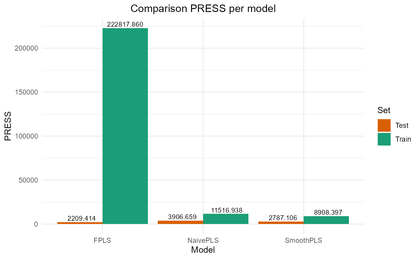
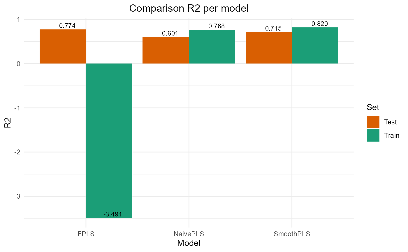
plot_model_metrics_base(train_results_f, test_results_f,
                        models_to_plot = c('FPLS', 'SmoothPLS'))