library(SmoothPLS)
library(pls)
#> Warning: package 'pls' was built under R version 4.4.3
#>
#> Attaching package: 'pls'
#> The following object is masked from 'package:stats':
#>
#>     loadings
This notebook show the Smooth PLS algorithm for a multi-states Categorical Functional Data (MS-CFD).
Parameters
N_states = 3

nind = 100 # number of individuals (train set)
start = 0 # First time
end = 100 # end time

curve_type = 'cat'

TTRatio = 0.2 # Train Test Ratio means we have floor(nind*TTRatio/(1-TTRatio))
NotS_ratio = 0.2 # noise variance over total variance for Y
beta_0_real=65.4321 # Intercept value for the link between X(t) and Y

nbasis = 10 # number of basis functions
norder = 4 # 4 for cubic splines basis

regul_time = seq(start, end, 5) # regularisation time sequence
regul_time_0 = seq(start, end, 1)

int_mode = 1 # in case of integration errors.
Data generation
lambda_determination
# Initialized the lambdas values
lambdas = lambda_determination(N_states)
lambdas
#> [1] 0.06615003 0.21686661 0.17015218
tranfer_probabilities
# Initialized the transition matrix
transition_df = transfer_probabilities(N_states)
transition_df
#>               dir1      dir2       dir3
#> state_1 0.00000000 0.0774743 0.92252570
#> state_2 0.95311191 0.0000000 0.04688809
#> state_3 0.08929956 0.9107004 0.00000000
df_cfd
df_cfd = generate_X_df_multistates(nind = nind, N_states, start, end,
                              lambdas,  transition_df)
head(df_cfd)
#>   id       time state
#> 1  1  0.0000000     3
#> 2  1  0.1855830     2
#> 3  1  0.6599301     1
#> 4  1  5.4101517     3
#> 5  1 21.4324942     2
#> 6  1 27.9593073     1
plot_CFD_individuals(df_cfd)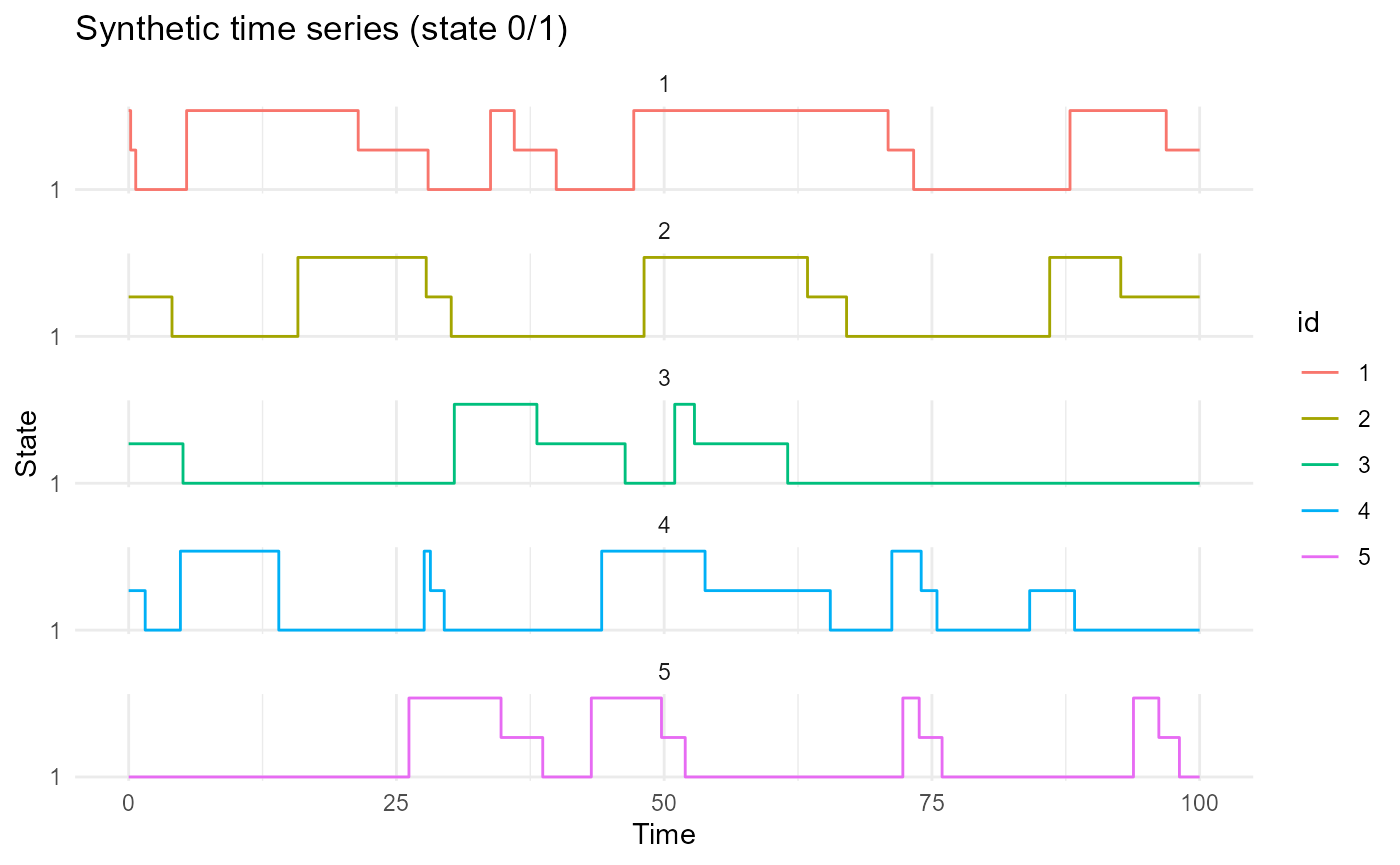
plot_CFD_individuals(df_cfd, by_cfda = TRUE)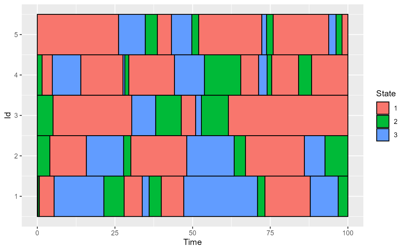
Basis creation
All the states will share the same basis.
basis = create_bspline_basis(start, end, nbasis, norder)
#basis = fda::create.fourier.basis(c(start,end), nbasis = nbasis)

# All the states will share the same basis.
basis_list = obj_list_creation(N_rep = N_states, obj = basis)

plot(basis, main=paste0(nbasis, " ", basis$type," functions basis"))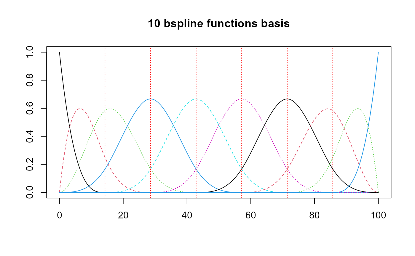
Data processing
We have to prepare the data before the FPLS method. For each state, we build its indicator function.
names(df_cfd)
#> [1] "id"    "time"  "state"
cat_data_to_indicator
df_processed = cat_data_to_indicator(df_cfd)

length(df_processed)
#> [1] 3
names(df_processed)
#> [1] "state_1" "state_2" "state_3"
head(df_processed$state_3, 20)
#>    id       time state
#> 1   1   0.000000     1
#> 2   1   0.185583     0
#> 4   1   5.410152     1
#> 5   1  21.432494     0
#> 7   1  33.788584     1
#> 8   1  36.004940     0
#> 10  1  47.160908     1
#> 11  1  70.910305     0
#> 13  1  87.895108     1
#> 14  1  96.879386     0
#> 15  1 100.000000     0
#> 16  2   0.000000     0
#> 18  2  15.802012     1
#> 19  2  27.782732     0
#> 21  2  48.123304     1
#> 22  2  63.385478     0
#> 24  2  85.998012     1
#> 25  2  92.634954     0
#> 26  2 100.000000     0
#> 27  3   0.000000     0
beta list
##### beta_real #####
###### beta_0_real ######
beta_0_real
#> [1] 65.4321
beta_func_list = beta_list_generation(N_states = N_states)
for(i in 1:length(beta_func_list)){
  plot(0:end,  beta_func_list[[i]](0:end, end_time = end),
       ylab=paste0("Beta(t) n°=", i), type = 'l')
  title(paste0("Beta(t) n°=", i))
}


Y evaluation
Y generation is based on the following equation : $Y = 0 + {i=1}^K _0^T _i(t) ind_i(t) dt $ with the indicator function of the state .
We link with the .
Y_df = generate_Y_df(df = df_processed, curve_type = curve_type,
                     beta_real_func_or_list =  beta_func_list,
                     beta_0_real = beta_0_real,
                     NotS_ratio = NotS_ratio)
#> Warning: package 'future' was built under R version 4.4.3
Y = Y_df$Y_noised
names(Y_df)
#> [1] "id"       "Y_beta1"  "Y_beta2"  "Y_beta3"  "Y_real"   "Y_noised"
head(Y_df)
#>   id  Y_beta1    Y_beta2      Y_beta3    Y_real  Y_noised
#> 1  1 29.21242   8.445168 -12.27938095  90.81031  91.70391
#> 2  2 29.33400  43.357133  -6.28448556 131.83875 133.47730
#> 3  3 61.59767 -32.556458   1.38131403  95.85463 117.59081
#> 4  4 21.89818  21.223380  -0.02003002 108.53363 114.37513
#> 5  5 56.99972   4.546594  -1.81193494 125.16648 109.13350
#> 6  6 18.74040  24.931901  -6.06344099 103.04096  94.33601
Test set
nind_test = floor(nind*TTRatio/(1-TTRatio))
df_test = generate_X_df_multistates(nind = nind_test, N_states, start, end,
                              lambdas,  transition_df)
df_test_processed = cat_data_to_indicator(df_test)

Y_df_test = generate_Y_df(df_test_processed, curve_type = curve_type,
                          beta_real_func_or_list = beta_func_list,
                          beta_0_real = beta_0_real,
                          NotS_ratio= NotS_ratio)
PLS functions
Naive PLS
naivePLS_obj = naivePLS(df_list = df_cfd, Y = Y, regul_time_obj = regul_time,
                        curve_type_obj = 'cat',
                        id_col_obj = 'id', time_col_obj = 'time',
                        print_steps = TRUE, plot_rmsep = TRUE,
                        print_nbComp = TRUE,plot_reg_curves = TRUE)
#> ### Naive PLS ###
#> => Input format assertions.
#> => Input format assertions OK.
#> => Data formatting.
#> => PLS model.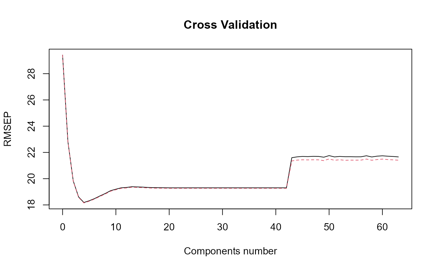
#> [1] "Optimal number of PLS components : 4"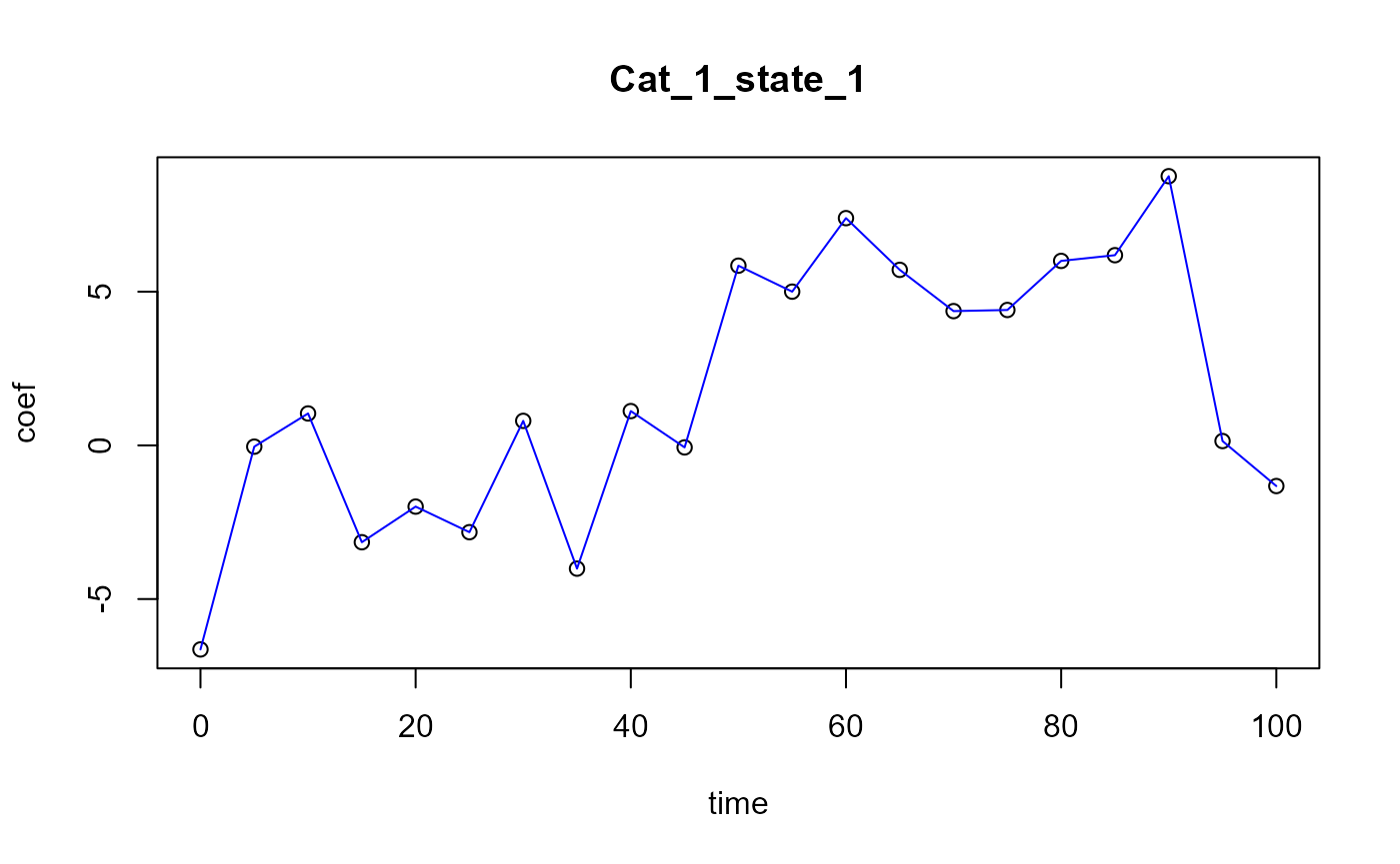
Functional PLS
fpls_obj = funcPLS(df_list = df_cfd, Y = Y_df$Y_noised,
                   basis_obj = basis,
                   curve_type_obj = 'cat',
                   regul_time_obj = regul_time,
                   id_col_obj = 'id', time_col_obj = 'time',
                   print_steps = TRUE, plot_rmsep = TRUE,
                   print_nbComp = TRUE, plot_reg_curves = TRUE)
#> ### Functional PLS ###
#> => Input format assertions.
#> => Input format assertions OK.
#> => Building alpha matrix.
#> => Building curve names.
#> ==> Evaluating alpha for : CatFD_1_1.
#>  ==> Evaluating alpha for : CatFD_1_2.
#>  ==> Evaluating alpha for : CatFD_1_3.
#> => Evaluate metrix and root_metric.
#> => plsr(Y ~ trans_alphas).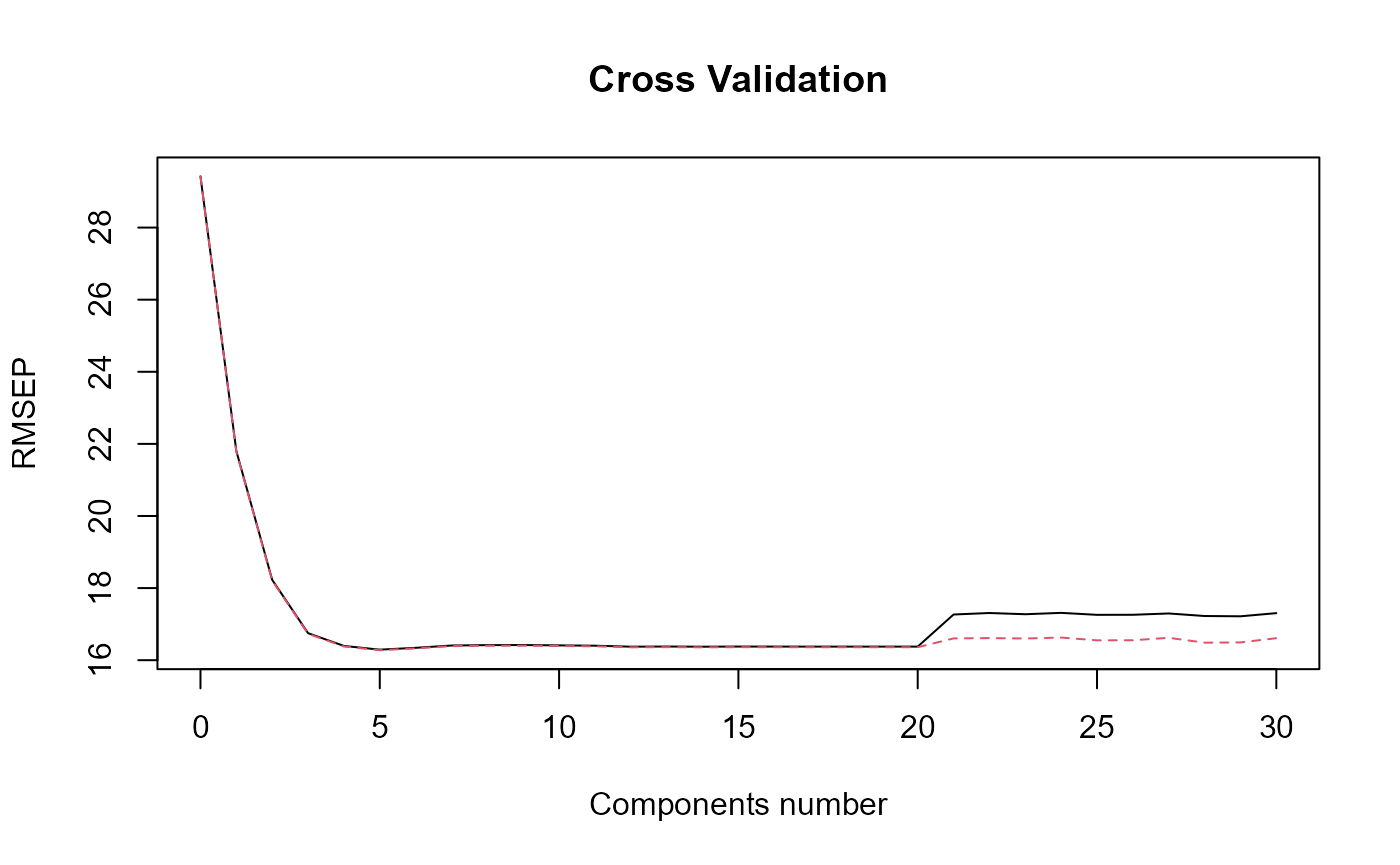
#> Optimal number of PLS components :  5 .
#> => Build Intercept and regression curves for optimal number of components.
#>  ==> Build  regression curve for : CatFD_1_1
#>  ==> Build  regression curve for : CatFD_1_2
#>  ==> Build  regression curve for : CatFD_1_3


Smooth PLS
spls_obj = smoothPLS(df_list = df_cfd, Y = Y_df$Y_noised, basis_obj = basis,
                     orth_obj = TRUE, curve_type_obj = 'cat',
                     int_mode = 1,
                     id_col_obj ='id', time_col_obj = 'time',
                     print_steps = TRUE, plot_rmsep = TRUE,
                     print_nbComp = TRUE, plot_reg_curves = TRUE)
#> ### Smooth PLS ###
#> ## Use parallelization in case of heavy computational load. ##
#> ## Threshold can be manualy adjusted : (default 2500) ##
#> ## >options(SmoothPLS.parallel_threshold = 500) ##
#> => Input format assertions.
#> => Input format assertions OK.
#> => Orthonormalize basis.
#> => Data objects formatting.
#> => Evaluate Lambda matrix.
#> ==> Lambda for : CatFD_1_state_1.
#> ==> Lambda for : CatFD_1_state_2.
#> ==> Lambda for : CatFD_1_state_3.
#> => PLSR model.
#> => Optimal number of PLS components : 8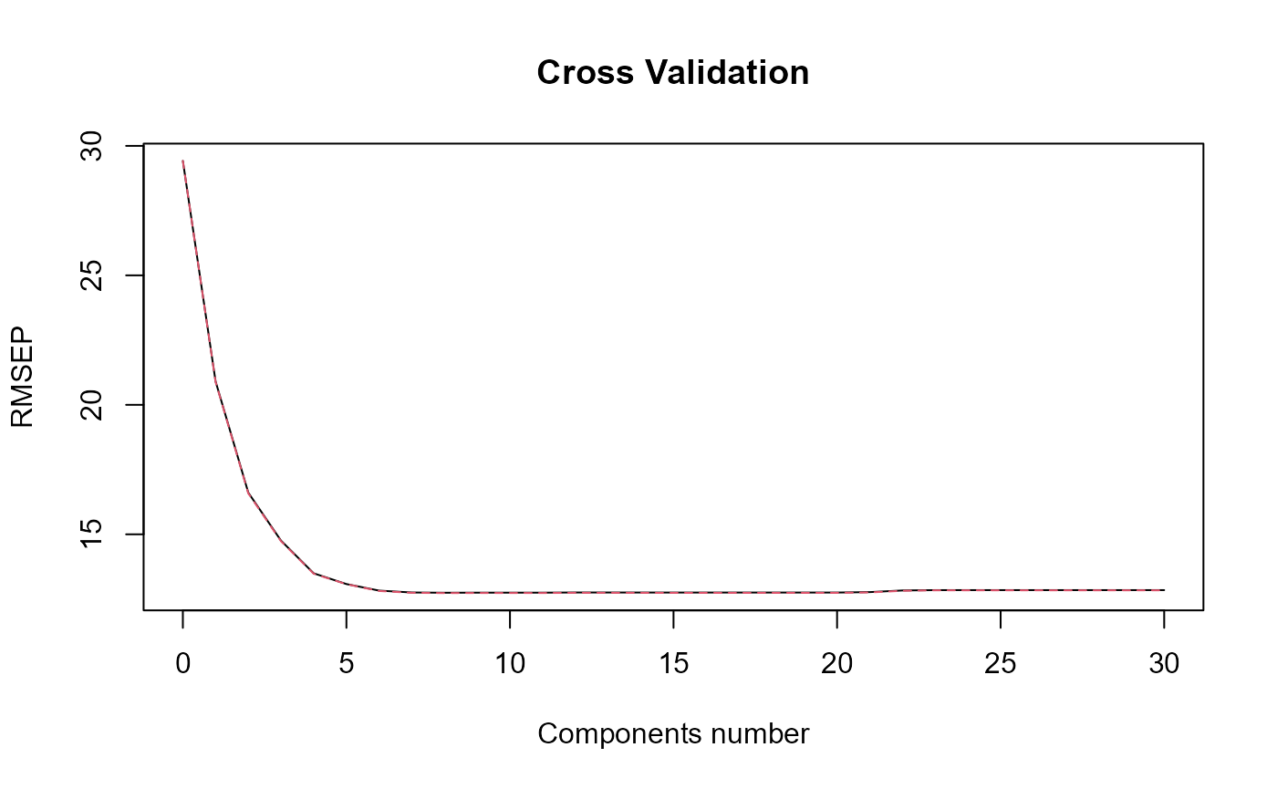
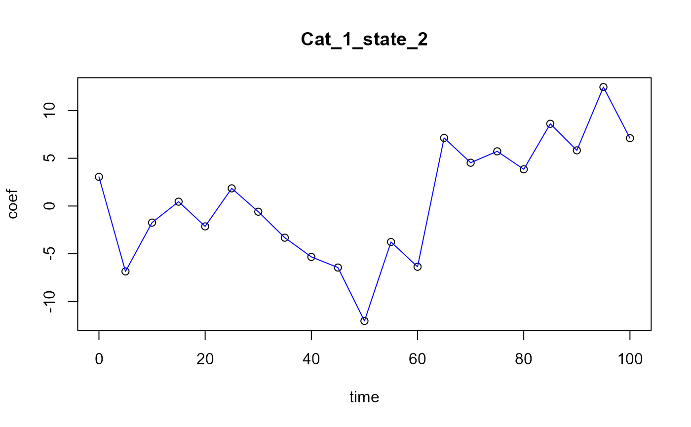
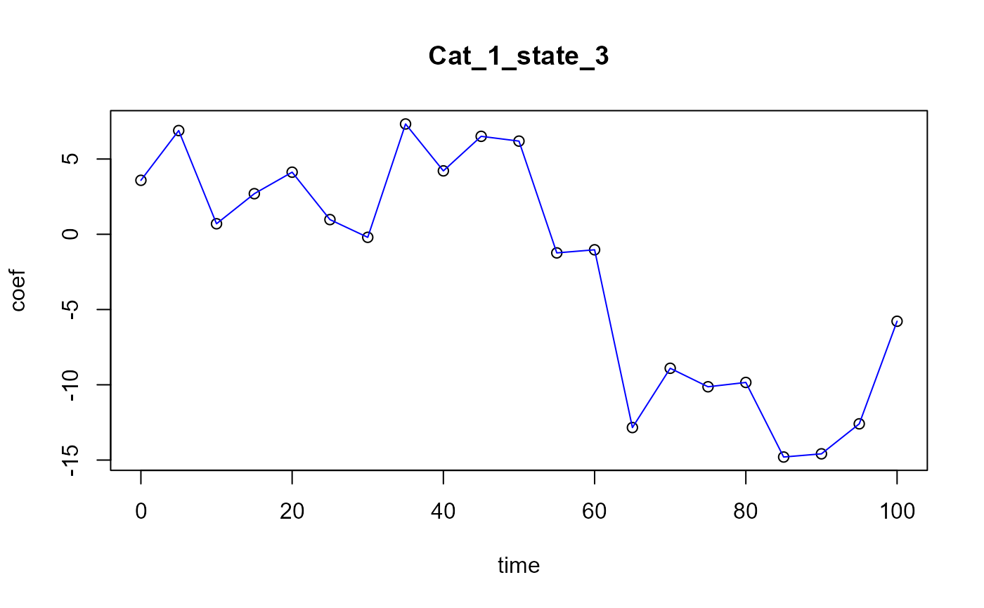
#> => Evaluate SmoothPLS functions and <w_i, p_j> coef.
#> => Build regression functions and intercept.
#> ==> Build regression curve for : CatFD_1_state_1
#> ==> Build regression curve for : CatFD_1_state_2
#> ==> Build regression curve for : CatFD_1_state_3


names(spls_obj$reg_obj)
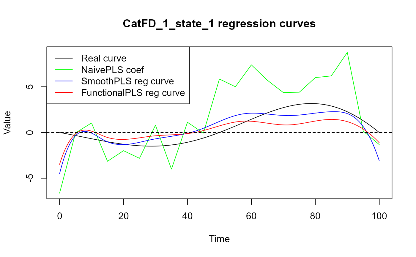
#> [1] "Intercept" "CatFD_1_state_1" "CatFD_1_state_2" "CatFD_1_state_3"Curves comparison
# Warning ms_spls_obj$delta_ms_list[[1]] is the intercept!
cat("curve_1 : smooth PLS regression curve.\n")
#> curve_1 : smooth PLS regression curve.
cat("curve_2 : functional PLS regression curve.\n")
#> curve_2 : functional PLS regression curve.
cat("curve_3 : naive PLS regression coefficients\n")
#> curve_3 : naive PLS regression coefficients
for(i in 1:N_states){
start = 0
print(paste0("State_", (i)))
evaluate_curves_distances(real_f = beta_func_list[[i]],
regul_time = regul_time,
fun_fd_list = list(spls_obj$reg_obj[[i+1]],
fpls_obj$reg_obj[[i+1]],
approxfun(
x = regul_time,
y = naivePLS_obj$opti_reg_coef[
start:(start+length(regul_time)
)])
)
)
start = start + length(regul_time)
}
#> [1] "State_1"
#> [1] "real_f -> curve_1 / INPROD : 3.72098051938215 / DIST : 11.4910155188119"
#> [1] "real_f -> curve_2 / INPROD : 25.0386959831357 / DIST : 12.396413572732"
#> [1] "real_f -> curve_3 / INPROD : -151.510446910693 / DIST : 32.9996112554268"
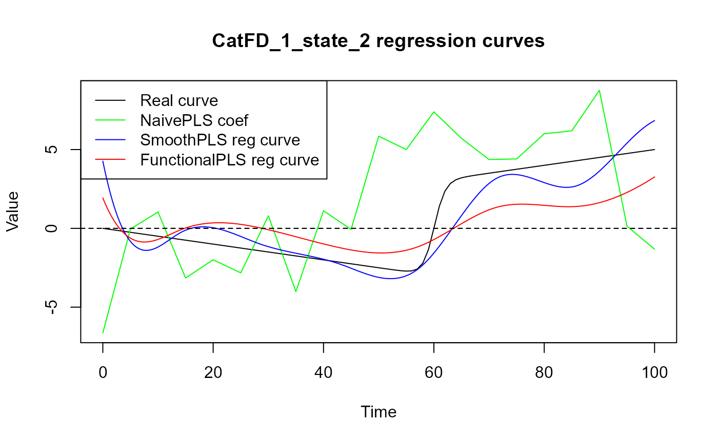
#> [1] "State_2"
#> [1] "real_f -> curve_1 / INPROD : 21.6384611829502 / DIST : 11.8442729473802"
#> [1] "real_f -> curve_2 / INPROD : 44.961118917043 / DIST : 17.9601660134444"
#> [1] "real_f -> curve_3 / INPROD : -133.512934779195 / DIST : 39.8105772928267"
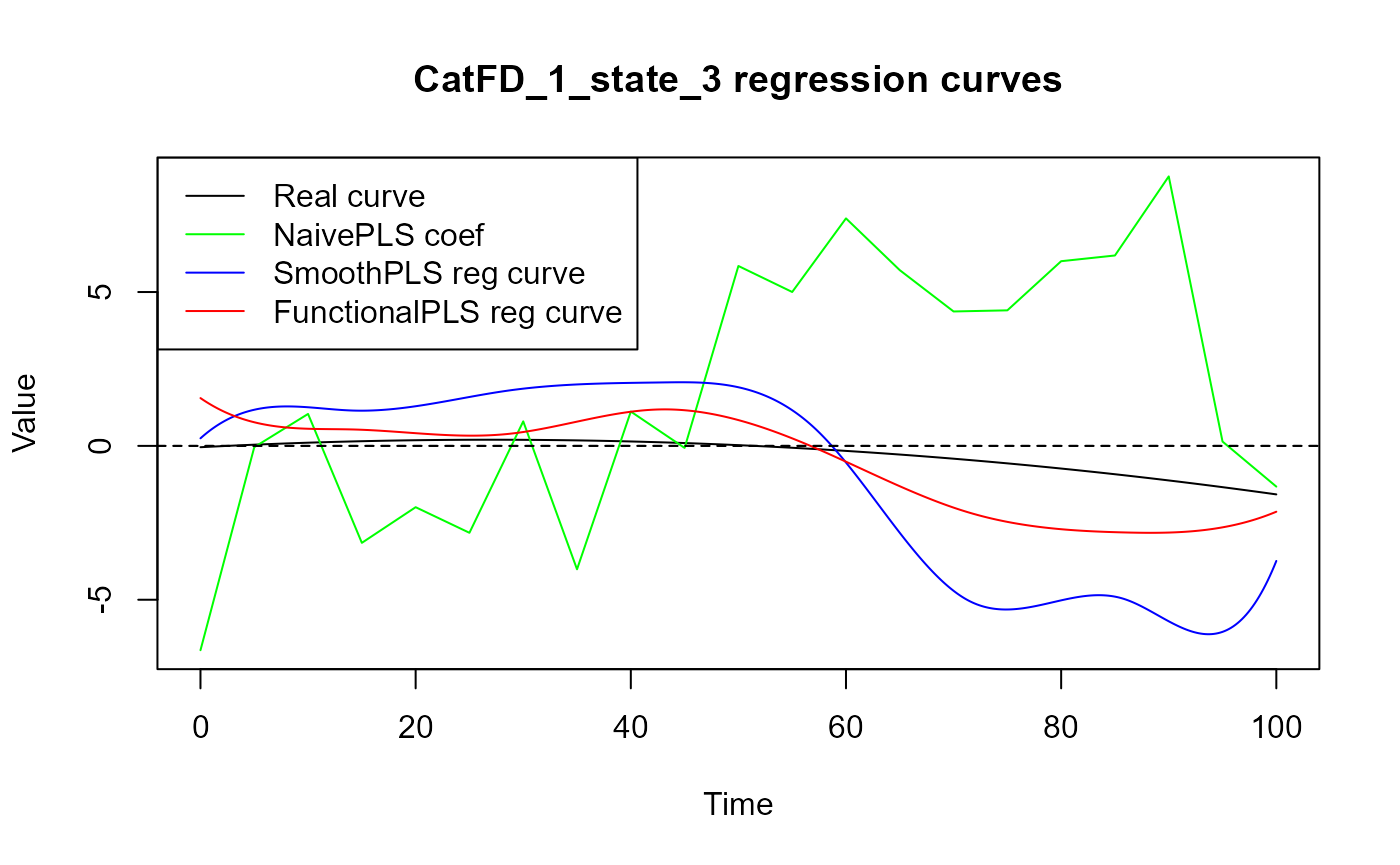
#> [1] "State_3"
#> [1] "real_f -> curve_1 / INPROD : 71.025199322987 / DIST : 27.6231009463399"
#> [1] "real_f -> curve_2 / INPROD : 26.3848272414933 / DIST : 11.1751571035391"
#> [1] "real_f -> curve_3 / INPROD : -229.02901191578 / DIST : 48.0770061426967"
for(i in 1:N_states){
  start = 0

  y_lim = eval_max_min_y(f_list = list(spls_obj$reg_ob[[i+1]],
                                       fpls_obj$reg_ob[[i+1]],
                                       approxfun(
                                         x = regul_time,
                                         y = naivePLS_obj$opti_reg_coef[
                                           start:(start+length(regul_time))]),
                                       beta_func_list[[i]]
                                       ),
                         regul_time = regul_time_0)

  plot(regul_time_0, beta_func_list[[i]](regul_time_0), col = 'black',
       ylim = y_lim, xlab = 'Time', ylab = 'Value', type = 'l')
  lines(regul_time_0, approxfun(x = regul_time,
                                y = naivePLS_obj$opti_reg_coef[
                                  start:(start+
                                           length(regul_time))])(regul_time_0),
       col = 'green')
  title(paste0(names(spls_obj$reg_obj)[i+1], " regression curves"))
  plot(spls_obj$reg_obj[[i+1]], col = 'blue', add = TRUE)
  plot(fpls_obj$reg_obj[[i+1]], col = 'red', add = TRUE)
  legend("topleft",
         legend = c("Real curve", "NaivePLS coef",
                    "SmoothPLS reg curve", "FunctionalPLS reg curve"),
         col = c("black", "green", "blue", "red"),
         lty = 1,
         lwd = 1)

  start = start + length(regul_time)
}
Results
train_results = data.frame(matrix(ncol = 5, nrow = 3))
colnames(train_results) = c("PRESS", "RMSE", "MAE", "R2", "var_Y")
rownames(train_results) = c("NaivePLS", "FPLS", "SmoothPLS")

test_results = train_resultsTrain set
Y_train = Y_df$Y_noised

# Naive
Y_hat = predict(naivePLS_obj$plsr_model,
                ncomp = naivePLS_obj$nbCP_opti,
                newdata = naivePLS_obj$plsr_model$model$`as.matrix(df_mod_wide)`)
train_results["NaivePLS", ] = evaluate_results(Y_train, Y_hat)


# FPLS
Y_hat_fpls = (predict(fpls_obj$plsr_model, ncomp = fpls_obj$nbCP_opti,
                newdata = fpls_obj$trans_alphas)
              + fpls_obj$reg_obj$Intercept
              + mean(Y))

Y_hat_fpls = smoothPLS_predict(df_predict_list = df_cfd,
                               delta_list = fpls_obj$reg_obj,
                               curve_type_obj = curve_type,
                               int_mode = int_mode,
                               regul_time_obj = regul_time)

train_results["FPLS", ] = evaluate_results(Y_train, Y_hat_fpls)

# Smooth PLS
Y_hat_spls = smoothPLS_predict(df_predict_list = df_cfd,
                               delta_list = spls_obj$reg_obj,
                               curve_type_obj = curve_type,
                               int_mode = int_mode,
                               regul_time_obj = regul_time)

train_results["SmoothPLS", ] = evaluate_results(Y_train, Y_hat_spls)

train_results["NaivePLS", "nb_cp"] = naivePLS_obj$nbCP_opti
train_results["FPLS", "nb_cp"] = fpls_obj$nbCP_opti
train_results["SmoothPLS", "nb_cp"] = spls_obj$nbCP_opti
train_results
#>              PRESS     RMSE       MAE        R2     var_Y nb_cp
#> NaivePLS  13559.18 11.64439  9.801626 0.8401608  84.01608     4
#> FPLS      13622.80 11.67167  9.407000 0.8394108  70.23009     5
#> SmoothPLS 73362.15 27.08545 21.832970 0.1351872 274.32359     8
Test set
Y_test = Y_df_test$Y_noised

# Naive
df_test_wide = naivePLS_formatting(df_list = df_test,
                                  regul_time_obj = regul_time,
                                  curve_type_obj = curve_type,
                                  id_col_obj = 'id', time_col_obj = 'time')

Y_hat = predict(naivePLS_obj$plsr_model,
                ncomp = naivePLS_obj$nbCP_opti,
                newdata = as.matrix(df_test_wide))
test_results["NaivePLS", ] = evaluate_results(Y_test, Y_hat)

# FPLS
Y_hat_fpls = smoothPLS_predict(df_predict_list = df_test,
                               delta_list = fpls_obj$reg_obj,
                               curve_type_obj = curve_type,
                               int_mode = int_mode,
                               regul_time_obj = regul_time)

test_results["FPLS", ] = evaluate_results(Y_test, Y_hat_fpls)

# Smooth PLS
Y_hat_spls = smoothPLS_predict(df_predict_list = df_test,
                               delta_list = spls_obj$reg_obj,
                               curve_type_obj = curve_type,
                               int_mode = int_mode,
                               regul_time_obj = regul_time)

test_results["SmoothPLS", ] = evaluate_results(Y_test, Y_hat_spls)

test_results["NaivePLS", "nb_cp"] = naivePLS_obj$nbCP_opti
test_results["FPLS", "nb_cp"] = fpls_obj$nbCP_opti
test_results["SmoothPLS", "nb_cp"] = spls_obj$nbCP_opti
test_results
#> PRESS RMSE MAE R2 var_Y nb_cp
#> NaivePLS 2145.521 9.263954 8.224727 0.8269473 109.30089 4
#> FPLS 1828.114 8.551291 6.671840 0.8525486 78.18203 5
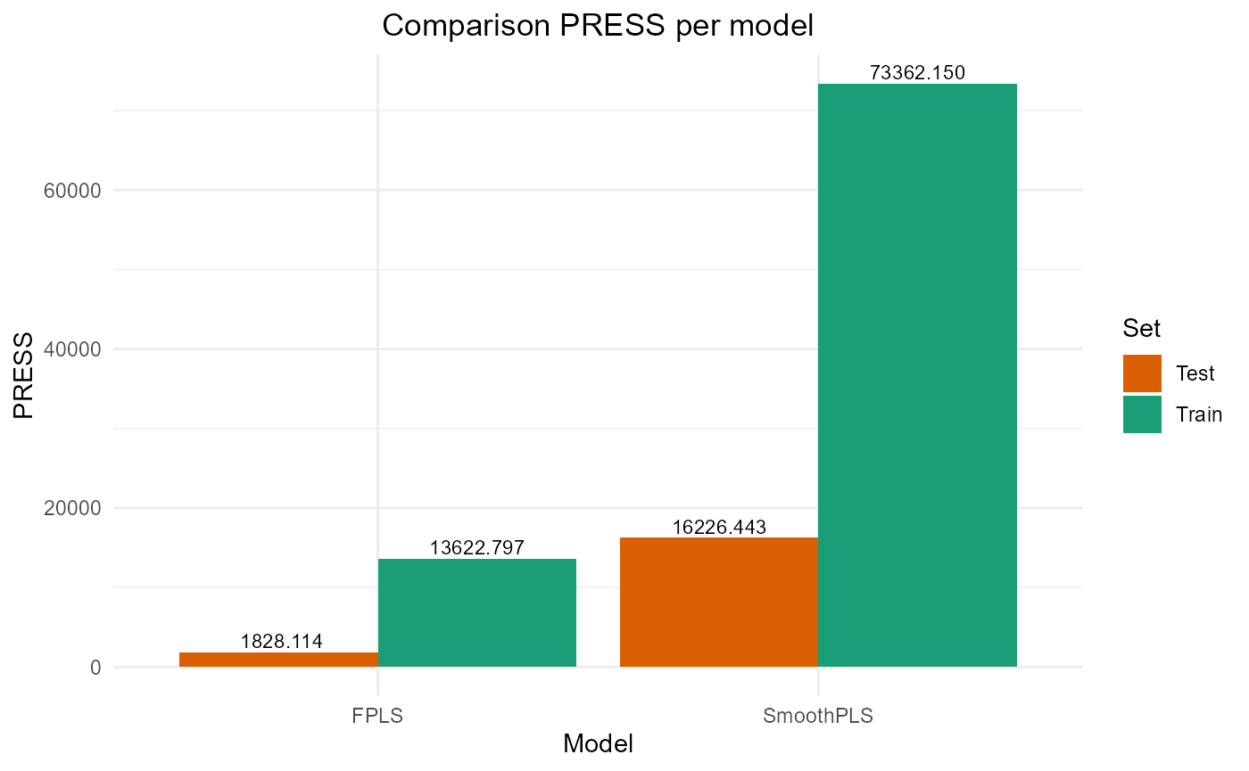
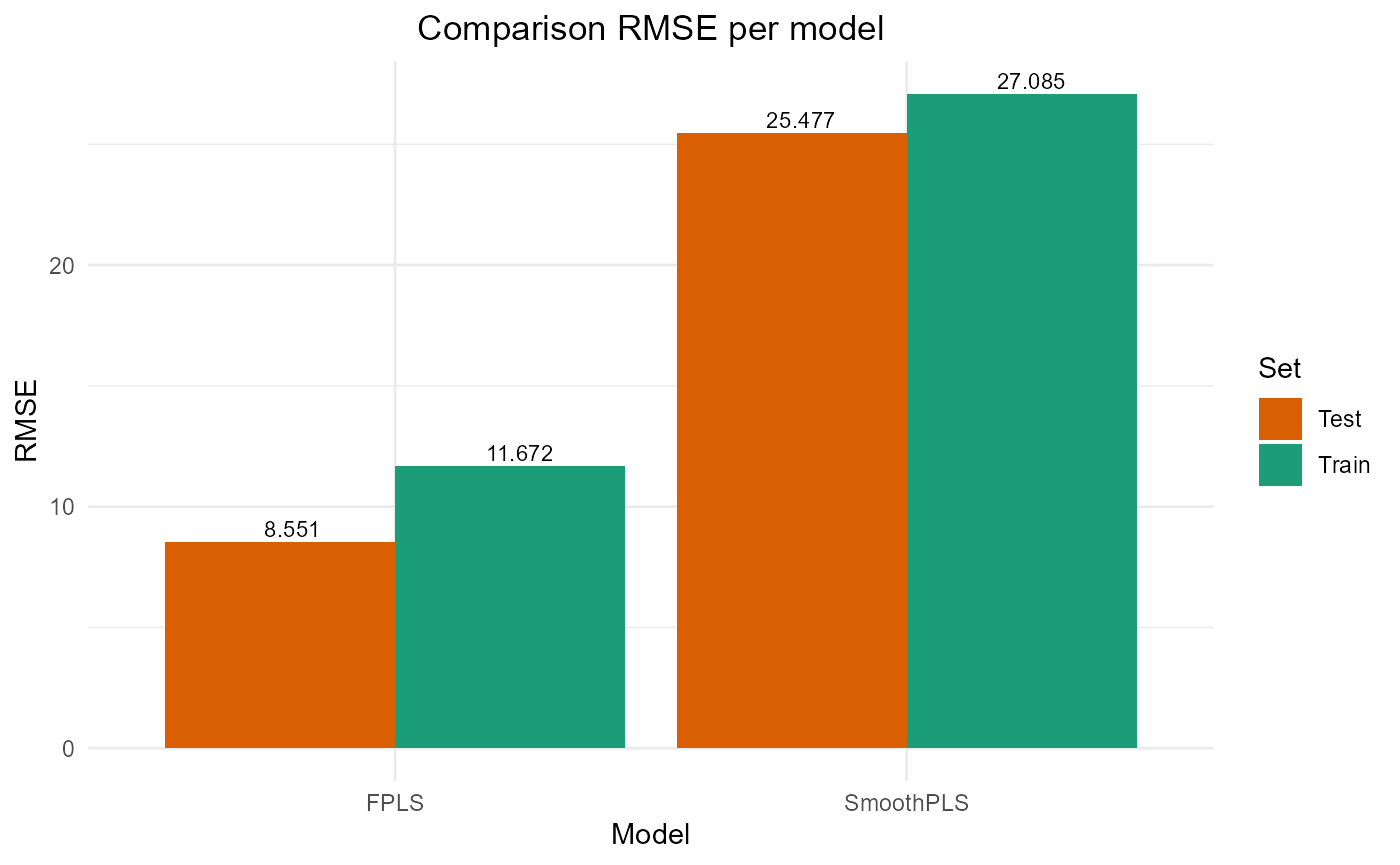
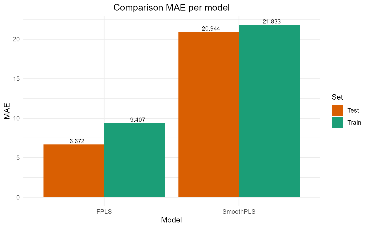
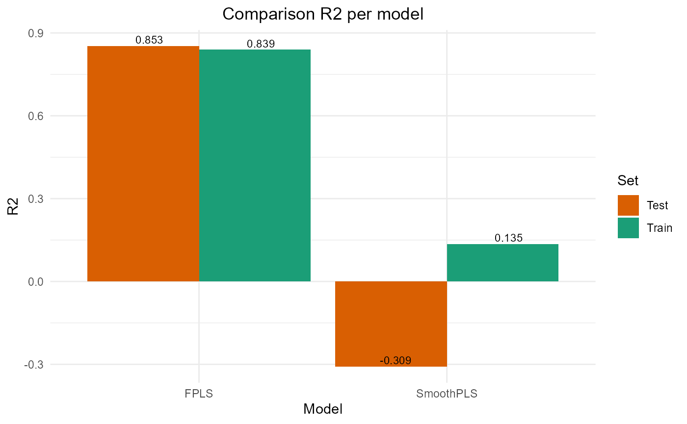
#> SmoothPLS 16226.443 25.476612 20.943841 -0.3087869 317.83813 8Plot results
train_results
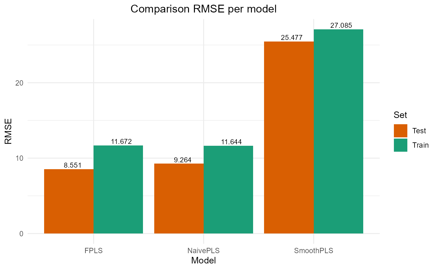
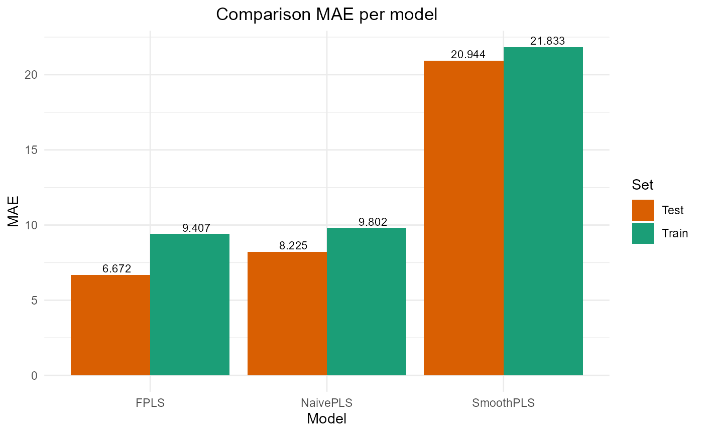
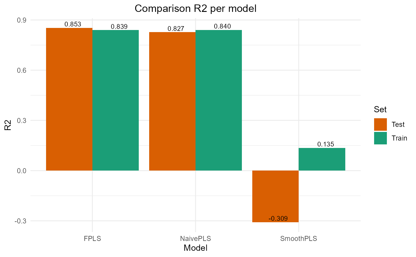
#> PRESS RMSE MAE R2 var_Y nb_cp
#> NaivePLS 13559.18 11.64439 9.801626 0.8401608 84.01608 4
#> FPLS 13622.80 11.67167 9.407000 0.8394108 70.23009 5
#> SmoothPLS 73362.15 27.08545 21.832970 0.1351872 274.32359 8
test_results
#> PRESS RMSE MAE R2 var_Y nb_cp
#> NaivePLS 2145.521 9.263954 8.224727 0.8269473 109.30089 4
#> FPLS 1828.114 8.551291 6.671840 0.8525486 78.18203 5
#> SmoothPLS 16226.443 25.476612 20.943841 -0.3087869 317.83813 8
plot_model_metrics_base(train_results, test_results)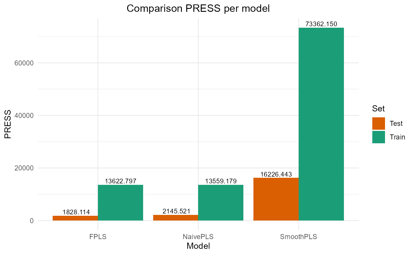
plot_model_metrics_base(train_results, test_results,
                        models_to_plot = c('FPLS', 'SmoothPLS'))